Fit of univariate distributions to non-censored data
fitdist.RdFit of univariate distributions to non-censored data by maximum likelihood (mle),
moment matching (mme), quantile matching (qme) or
maximizing goodness-of-fit estimation (mge).
The latter is also known as minimizing distance estimation.
Generic methods are print, plot,
summary, quantile, logLik, AIC,
BIC, vcov and coef.
Usage
fitdist(data, distr, method = c("mle", "mme", "qme", "mge", "mse"),
    start=NULL, fix.arg=NULL, discrete, keepdata = TRUE, keepdata.nb=100,
    calcvcov=TRUE, ...)

# S3 method for class 'fitdist'
print(x, ...)

# S3 method for class 'fitdist'
plot(x, breaks="default", ...)

# S3 method for class 'fitdist'
summary(object, ...)

# S3 method for class 'fitdist'
logLik(object, ...)

# S3 method for class 'fitdist'
AIC(object, ..., k = 2)

# S3 method for class 'fitdist'
BIC(object, ...)

# S3 method for class 'fitdist'
vcov(object, ...)

# S3 method for class 'fitdist'
coef(object, ...)
Arguments
- data
A numeric vector.
- distr
A character string
"name"naming a distribution for which the corresponding density functiondname, the corresponding distribution functionpnameand the corresponding quantile functionqnamemust be defined, or directly the density function.- method
A character string coding for the fitting method:
"mle"for 'maximum likelihood estimation',"mme"for 'moment matching estimation',"qme"for 'quantile matching estimation',"mge"for 'maximum goodness-of-fit estimation' and"mse"for 'maximum spacing estimation'.- start
A named list giving the initial values of parameters of the named distribution or a function of data computing initial values and returning a named list. This argument may be omitted (default) for some distributions for which reasonable starting values are computed (see the 'details' section of
mledist). It may not be into account for closed-form formulas.- fix.arg
An optional named list giving the values of fixed parameters of the named distribution or a function of data computing (fixed) parameter values and returning a named list. Parameters with fixed value are thus NOT estimated by this maximum likelihood procedure. The use of this argument is not possible if
method="mme"and a closed-form formula is used.- keepdata
a logical. If
TRUE, dataset is returned, otherwise only a sample subset is returned.- keepdata.nb
When
keepdata=FALSE, the length (>1) of the subset returned.- calcvcov
A logical indicating if (asymptotic) covariance matrix is required.
- discrete
If TRUE, the distribution is considered as discrete. If
discreteis missing,discreteis automaticaly set toTRUEwhendistrbelongs to"binom","nbinom","geom","hyper"or"pois"and toFALSEin the other cases. It is thus recommended to enter this argument when using another discrete distribution. This argument will not directly affect the results of the fit but will be passed to functionsgofstat,plotdistandcdfcomp.- x
An object of class
"fitdist".- object
An object of class
"fitdist".- breaks
If
"default"the histogram is plotted with the functionhistwith its default breaks definition. Elsebreaksis passed to the functionhist. This argument is not taken into account with discrete distributions:"binom","nbinom","geom","hyper"and"pois".- k
penalty per parameter to be passed to the AIC generic function (2 by default).
- ...
Further arguments to be passed to generic functions, or to one of the functions
"mledist","mmedist","qmedist"or"mgedist"depending of the chosen method. Seemledist,mmedist,qmedist,mgedistfor details on parameter estimation.
Details
It is assumed that the distr argument specifies the distribution by the
probability density function, the cumulative distribution function and
the quantile function (d, p, q).
The four possible fitting methods are described below:
- When
method="mle" Maximum likelihood estimation consists in maximizing the log-likelihood. A numerical optimization is carried out in
mledistviaoptimto find the best values (seemledistfor details).- When
method="mme" Moment matching estimation consists in equalizing theoretical and empirical moments. Estimated values of the distribution parameters are computed by a closed-form formula for the following distributions :
"norm","lnorm","pois","exp","gamma","nbinom","geom","beta","unif"and"logis". Otherwise the theoretical and the empirical moments are matched numerically, by minimization of the sum of squared differences between observed and theoretical moments. In this last case, further arguments are needed in the call tofitdist:orderandmemp(seemmedistfor details).Since Version 1.2-0,
mmedistautomatically computes the asymptotic covariance matrix, hence the theoretical momentsmdistshould be defined up to an order which equals to twice the maximal order givenorder.- When
method = "qme" Quantile matching estimation consists in equalizing theoretical and empirical quantile. A numerical optimization is carried out in
qmedistviaoptimto minimize of the sum of squared differences between observed and theoretical quantiles. The use of this method requires an additional argumentprobs, defined as the numeric vector of the probabilities for which the quantile(s) is(are) to be matched (seeqmedistfor details).- When
method = "mge" Maximum goodness-of-fit estimation consists in maximizing a goodness-of-fit statistics. A numerical optimization is carried out in
mgedistviaoptimto minimize the goodness-of-fit distance. The use of this method requires an additional argumentgofcoding for the goodness-of-fit distance chosen. One can use the classical Cramer-von Mises distance ("CvM"), the classical Kolmogorov-Smirnov distance ("KS"), the classical Anderson-Darling distance ("AD") which gives more weight to the tails of the distribution, or one of the variants of this last distance proposed by Luceno (2006) (seemgedistfor more details). This method is not suitable for discrete distributions.- When
method = "mse" Maximum goodness-of-fit estimation consists in maximizing the average log spacing. A numerical optimization is carried out in
msedistviaoptim.
By default, direct optimization of the log-likelihood (or other criteria depending
of the chosen method) is performed using optim,
with the "Nelder-Mead" method for distributions characterized by more than one parameter
and the "BFGS" method for distributions characterized by only one parameter.
The optimization algorithm used in optim can be chosen or another optimization function
can be specified using ... argument (see mledist for details).
start may be omitted (i.e. NULL) for some classic distributions
(see the 'details' section of mledist).
Note that when errors are raised by optim, it's a good idea to start by adding traces during
the optimization process by adding control=list(trace=1, REPORT=1) in ... argument.
Once the parameter(s) is(are) estimated, fitdist computes the log-likelihood
for every estimation method and for maximum likelihood estimation the standard errors of
the estimates calculated from the Hessian at the solution found by optim
or by the user-supplied function passed to mledist.
By default (keepdata = TRUE), the object returned by fitdist contains
the data vector given in input.
When dealing with large datasets, we can remove the original dataset from the output by
setting keepdata = FALSE. In such a case, only keepdata.nb points (at most)
are kept by random subsampling keepdata.nb-2 points from the dataset and
adding the minimum and the maximum. If combined with bootdist, and use with
non-parametric bootstrap be aware that bootstrap is performed on the subset
randomly selected in fitdist. Currently, the graphical comparisons of multiple fits
is not available in this framework.
Weighted version of the estimation process is available for method = "mle", "mme", "qme"
by using weights=.... See the corresponding man page for details.
Weighted maximum GOF estimation (when method = "mge") is not allowed.
It is not yet possible to take into account weighths in functions plotdist,
plot.fitdist, cdfcomp, denscomp, ppcomp,
qqcomp, gofstat and descdist (developments planned in the future).
Once the parameter(s) is(are) estimated, gofstat allows to compute
goodness-of-fit statistics.
NB: if your data values are particularly small or large, a scaling may be needed
before the optimization process. See example (14) in this man page and
examples (14,15) in the test file of the package.
Please also take a look at the Rmpfr package available on CRAN for numerical
accuracy issues.
Value
fitdist returns an object of class "fitdist", a list with the following components:
- estimate
the parameter estimates.
- method
the character string coding for the fitting method :
"mle"for 'maximum likelihood estimation',"mme"for 'matching moment estimation',"qme"for 'matching quantile estimation'"mge"for 'maximum goodness-of-fit estimation' and"mse"for 'maximum spacing estimation'.- sd
the estimated standard errors,
NAif numerically not computable orNULLif not available.- cor
the estimated correlation matrix,
NAif numerically not computable orNULLif not available.- vcov
the estimated variance-covariance matrix,
NULLif not available for the estimation method considered.- loglik
the log-likelihood.
- aic
the Akaike information criterion.
- bic
the the so-called BIC or SBC (Schwarz Bayesian criterion).
- n
the length of the data set.
- data
the data set.
- distname
the name of the distribution.
- fix.arg
the named list giving the values of parameters of the named distribution that must be kept fixed rather than estimated by maximum likelihood or
NULLif there are no such parameters.- fix.arg.fun
the function used to set the value of
fix.argorNULL.- dots
the list of further arguments passed in ... to be used in
bootdistin iterative calls tomledist,mmedist,qmedist,mgedistorNULLif no such arguments.- convergence
an integer code for the convergence of
optim/constrOptimdefined as below or defined by the user in the user-supplied optimization function.0indicates successful convergence.1indicates that the iteration limit ofoptimhas been reached.10indicates degeneracy of the Nealder-Mead simplex.100indicates thatoptimencountered an internal error.- discrete
the input argument or the automatic definition by the function to be passed to functions
gofstat,plotdistandcdfcomp.- weights
the vector of weigths used in the estimation process or
NULL.
Generic functions:
printThe print of a
"fitdist"object shows few traces about the fitting method and the fitted distribution.summaryThe summary provides the parameter estimates of the fitted distribution, the log-likelihood, AIC and BIC statistics and when the maximum likelihood is used, the standard errors of the parameter estimates and the correlation matrix between parameter estimates.
plotThe plot of an object of class "fitdist" returned by
fitdistuses the functionplotdist. An object of class "fitdist" or a list of objects of class "fitdist" corresponding to various fits using the same data set may also be plotted using a cdf plot (functioncdfcomp), a density plot(functiondenscomp), a density Q-Q plot (functionqqcomp), or a P-P plot (functionppcomp).logLikExtracts the estimated log-likelihood from the
"fitdist"object.AICExtracts the AIC from the
"fitdist"object.BICExtracts the estimated BIC from the
"fitdist"object.vcovExtracts the estimated var-covariance matrix from the
"fitdist"object (only available Whenmethod = "mle").coefExtracts the fitted coefficients from the
"fitdist"object.
See also
See fitdistrplus for an overview of the package.
See mledist, mmedist, qmedist,
mgedist, msedist for details on parameter estimation.
See gofstat for goodness-of-fit statistics.
See plotdist, graphcomp, CIcdfplot for graphs
(with or without uncertainty and/or multiple fits).
See llplot for (log-)likelihood plots in the
neighborhood of the fitted value.
See bootdist for bootstrap procedures
and fitdistcens for censored-data fitting methods.
See optim for base R optimization procedures.
See quantile.fitdist, another generic function, which calculates
quantiles from the fitted distribution.
See quantile for base R quantile computation.
Please visit the Frequently Asked Questions.
References
I. Ibragimov and R. Has'minskii (1981), Statistical Estimation - Asymptotic Theory, Springer-Verlag, doi:10.1007/978-1-4899-0027-2
Cullen AC and Frey HC (1999), Probabilistic techniques in exposure assessment. Plenum Press, USA, pp. 81-155.
Venables WN and Ripley BD (2002), Modern applied statistics with S. Springer, New York, pp. 435-446, doi:10.1007/978-0-387-21706-2 .
Vose D (2000), Risk analysis, a quantitative guide. John Wiley & Sons Ltd, Chischester, England, pp. 99-143.
Delignette-Muller ML and Dutang C (2015), fitdistrplus: An R Package for Fitting Distributions. Journal of Statistical Software, 64(4), 1-34, doi:10.18637/jss.v064.i04 .
Examples
set.seed(123) # here just to make random sampling reproducible
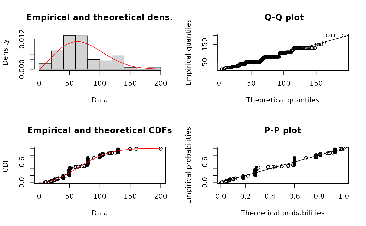
# (1) fit of a gamma distribution by maximum likelihood estimation
#
data(groundbeef)
serving <- groundbeef$serving
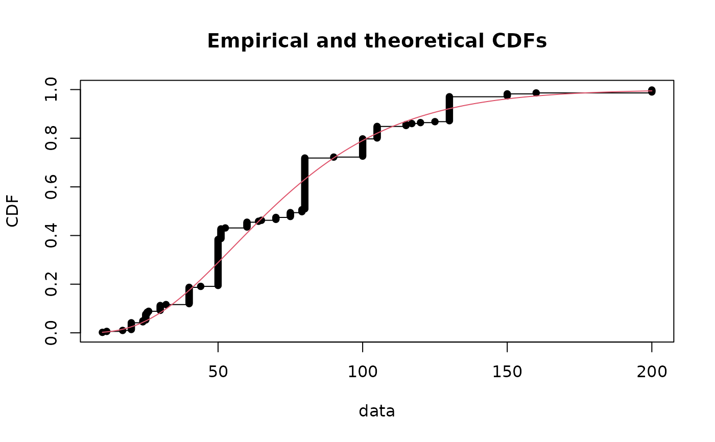
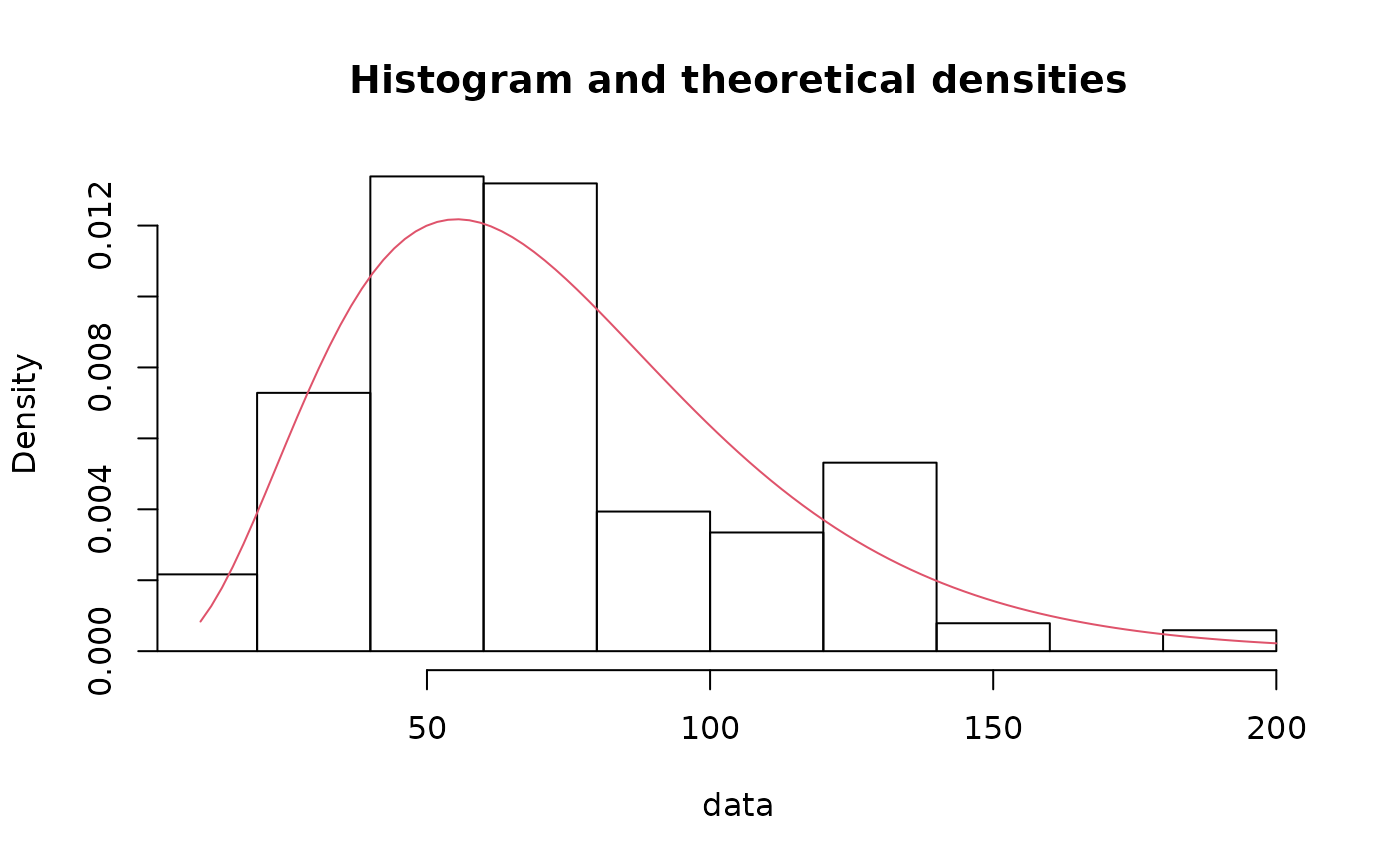
fitg <- fitdist(serving, "gamma")
summary(fitg)
#> Fitting of the distribution ' gamma ' by maximum likelihood
#> Parameters :
#> estimate Std. Error
#> shape 4.00955898 0.341451640
#> rate 0.05443907 0.004937239
#> Loglikelihood: -1253.625 AIC: 2511.25 BIC: 2518.325
#> Correlation matrix:
#> shape rate
#> shape 1.0000000 0.9384578
#> rate 0.9384578 1.0000000
#>
plot(fitg)
 plot(fitg, demp = TRUE)
 plot(fitg, histo = FALSE, demp = TRUE)
 cdfcomp(fitg, addlegend=FALSE)
 denscomp(fitg, addlegend=FALSE)
 ppcomp(fitg, addlegend=FALSE)
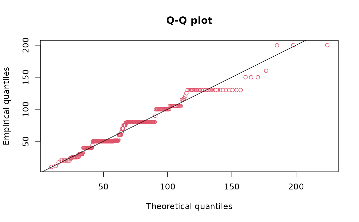
 qqcomp(fitg, addlegend=FALSE)
 # (2) use the moment matching estimation (using a closed formula)
#
fitgmme <- fitdist(serving, "gamma", method="mme")
summary(fitgmme)
#> Fitting of the distribution ' gamma ' by matching moments
#> Parameters :
#> estimate Std. Error
#> shape 4.22848617 0.417232914
#> rate 0.05741663 0.005930118
#> Loglikelihood: -1253.825 AIC: 2511.65 BIC: 2518.724
#> Correlation matrix:
#> shape rate
#> shape 1.0000000 0.9553622
#> rate 0.9553622 1.0000000
#>
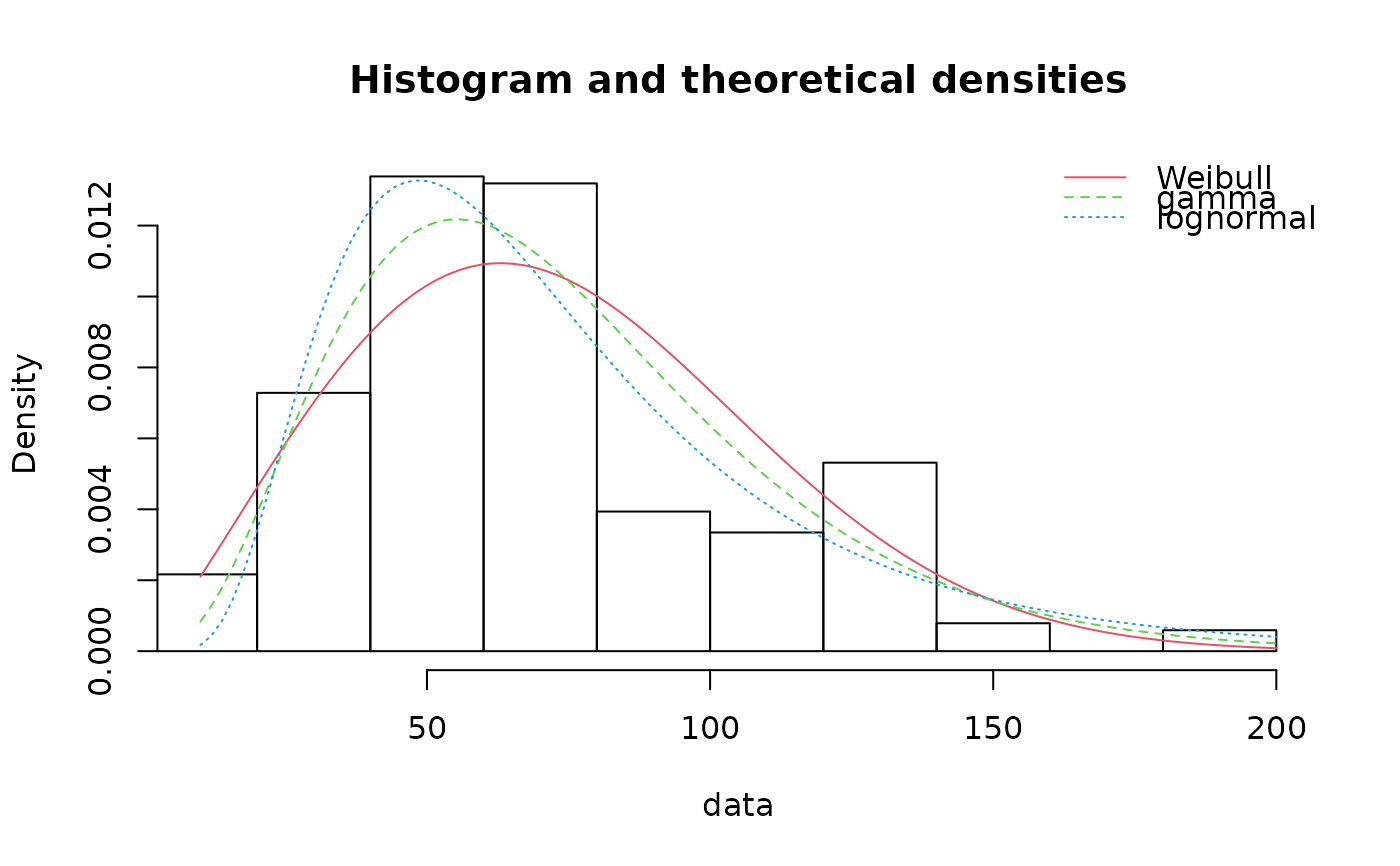
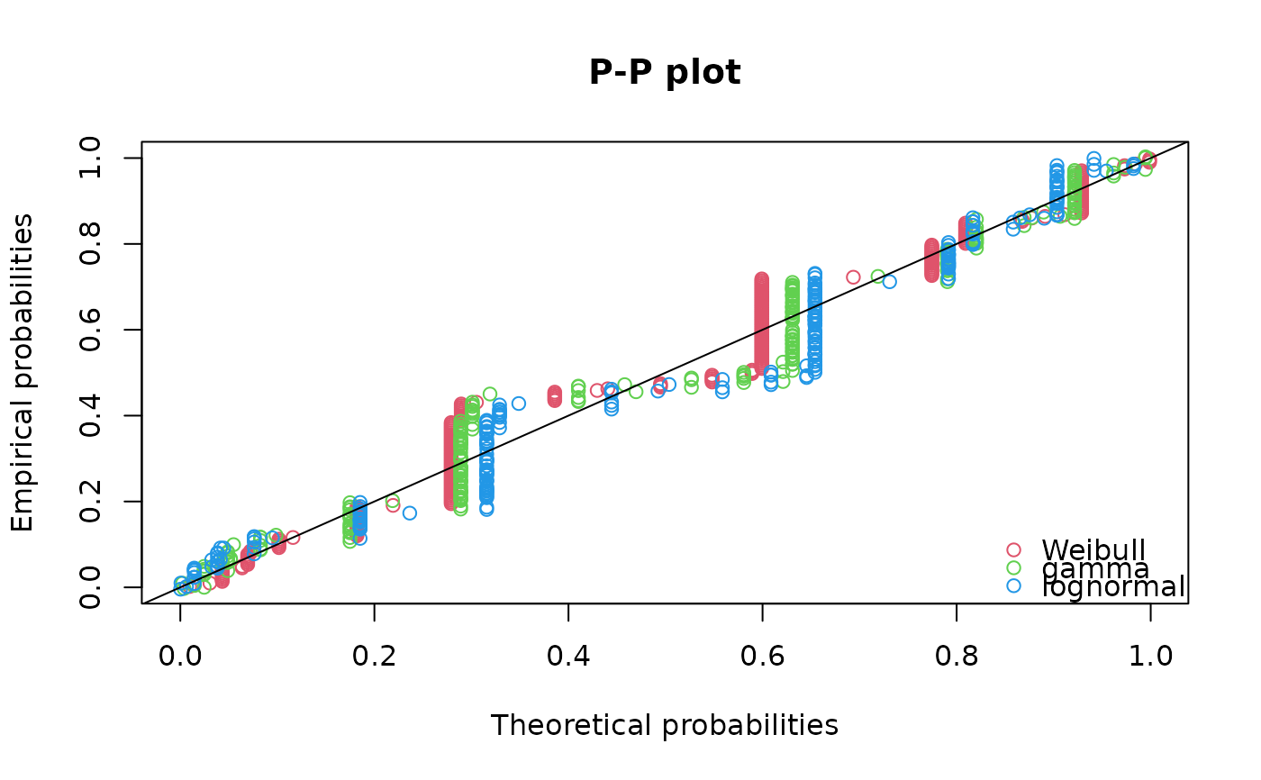
# (3) Comparison of various fits
#
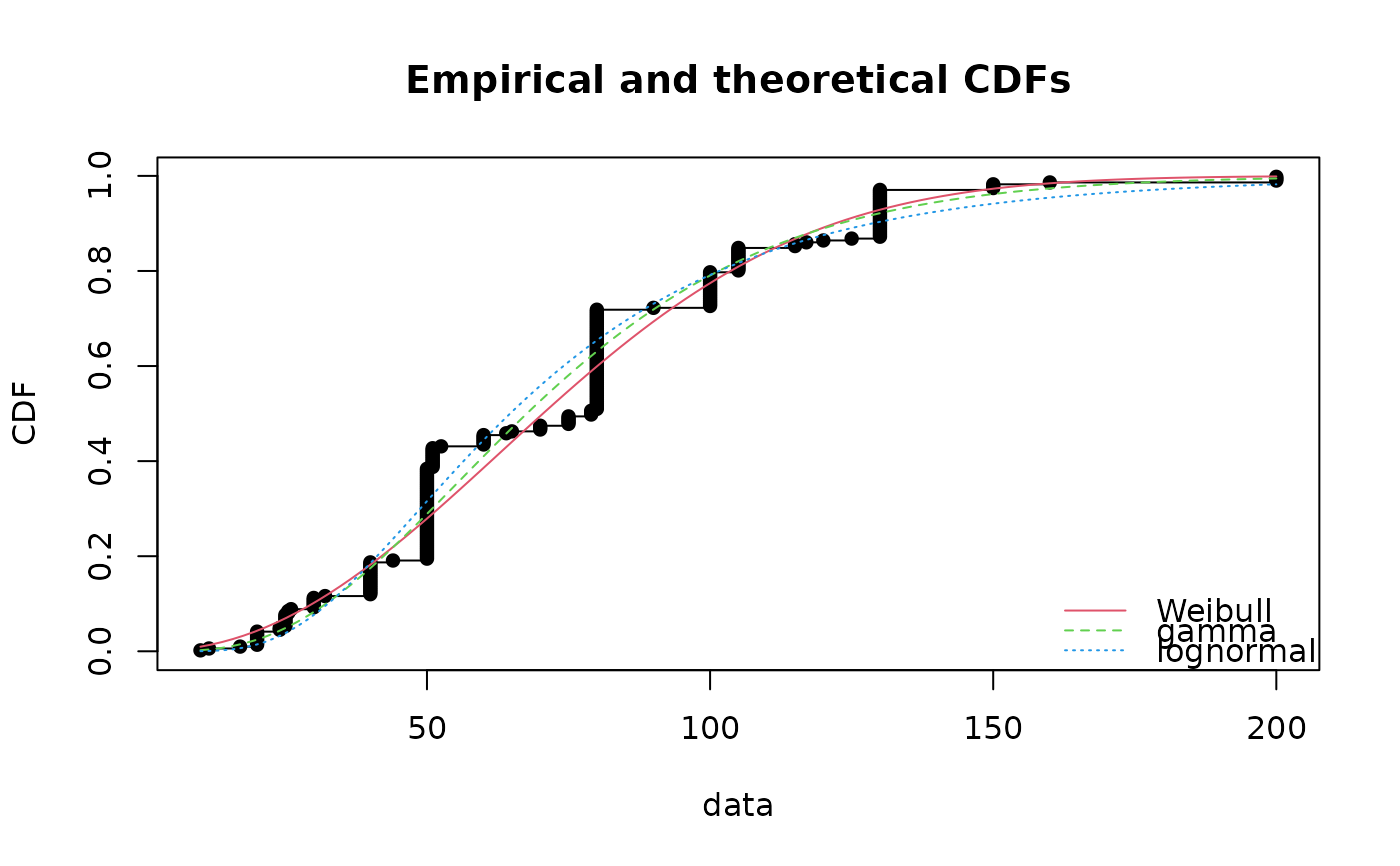
fitW <- fitdist(serving, "weibull")
fitg <- fitdist(serving, "gamma")
fitln <- fitdist(serving, "lnorm")
summary(fitW)
#> Fitting of the distribution ' weibull ' by maximum likelihood
#> Parameters :
#> estimate Std. Error
#> shape 2.185885 0.1045755
#> scale 83.347679 2.5268631
#> Loglikelihood: -1255.225 AIC: 2514.449 BIC: 2521.524
#> Correlation matrix:
#> shape scale
#> shape 1.000000 0.321821
#> scale 0.321821 1.000000
#>
summary(fitg)
#> Fitting of the distribution ' gamma ' by maximum likelihood
#> Parameters :
#> estimate Std. Error
#> shape 4.00955898 0.341451640
#> rate 0.05443907 0.004937239
#> Loglikelihood: -1253.625 AIC: 2511.25 BIC: 2518.325
#> Correlation matrix:
#> shape rate
#> shape 1.0000000 0.9384578
#> rate 0.9384578 1.0000000
#>
summary(fitln)
#> Fitting of the distribution ' lnorm ' by maximum likelihood
#> Parameters :
#> estimate Std. Error
#> meanlog 4.1693701 0.03366988
#> sdlog 0.5366095 0.02380783
#> Loglikelihood: -1261.319 AIC: 2526.639 BIC: 2533.713
#> Correlation matrix:
#> meanlog sdlog
#> meanlog 1 0
#> sdlog 0 1
#>
cdfcomp(list(fitW, fitg, fitln), legendtext=c("Weibull", "gamma", "lognormal"))
# (2) use the moment matching estimation (using a closed formula)
#
fitgmme <- fitdist(serving, "gamma", method="mme")
summary(fitgmme)
#> Fitting of the distribution ' gamma ' by matching moments
#> Parameters :
#> estimate Std. Error
#> shape 4.22848617 0.417232914
#> rate 0.05741663 0.005930118
#> Loglikelihood: -1253.825 AIC: 2511.65 BIC: 2518.724
#> Correlation matrix:
#> shape rate
#> shape 1.0000000 0.9553622
#> rate 0.9553622 1.0000000
#>
# (3) Comparison of various fits
#
fitW <- fitdist(serving, "weibull")
fitg <- fitdist(serving, "gamma")
fitln <- fitdist(serving, "lnorm")
summary(fitW)
#> Fitting of the distribution ' weibull ' by maximum likelihood
#> Parameters :
#> estimate Std. Error
#> shape 2.185885 0.1045755
#> scale 83.347679 2.5268631
#> Loglikelihood: -1255.225 AIC: 2514.449 BIC: 2521.524
#> Correlation matrix:
#> shape scale
#> shape 1.000000 0.321821
#> scale 0.321821 1.000000
#>
summary(fitg)
#> Fitting of the distribution ' gamma ' by maximum likelihood
#> Parameters :
#> estimate Std. Error
#> shape 4.00955898 0.341451640
#> rate 0.05443907 0.004937239
#> Loglikelihood: -1253.625 AIC: 2511.25 BIC: 2518.325
#> Correlation matrix:
#> shape rate
#> shape 1.0000000 0.9384578
#> rate 0.9384578 1.0000000
#>
summary(fitln)
#> Fitting of the distribution ' lnorm ' by maximum likelihood
#> Parameters :
#> estimate Std. Error
#> meanlog 4.1693701 0.03366988
#> sdlog 0.5366095 0.02380783
#> Loglikelihood: -1261.319 AIC: 2526.639 BIC: 2533.713
#> Correlation matrix:
#> meanlog sdlog
#> meanlog 1 0
#> sdlog 0 1
#>
cdfcomp(list(fitW, fitg, fitln), legendtext=c("Weibull", "gamma", "lognormal"))
 denscomp(list(fitW, fitg, fitln), legendtext=c("Weibull", "gamma", "lognormal"))
 qqcomp(list(fitW, fitg, fitln), legendtext=c("Weibull", "gamma", "lognormal"))
 ppcomp(list(fitW, fitg, fitln), legendtext=c("Weibull", "gamma", "lognormal"))
 gofstat(list(fitW, fitg, fitln), fitnames=c("Weibull", "gamma", "lognormal"))
#> Goodness-of-fit statistics
#> Weibull gamma lognormal
#> Kolmogorov-Smirnov statistic 0.1396646 0.1281486 0.1493090
#> Cramer-von Mises statistic 0.6840994 0.6936274 0.8277358
#> Anderson-Darling statistic 3.5736460 3.5672625 4.5436542
#>
#> Goodness-of-fit criteria
#> Weibull gamma lognormal
#> Akaike's Information Criterion 2514.449 2511.250 2526.639
#> Bayesian Information Criterion 2521.524 2518.325 2533.713
# (4) defining your own distribution functions, here for the Gumbel distribution
# for other distributions, see the CRAN task view
# dedicated to probability distributions
#
dgumbel <- function(x, a, b) 1/b*exp((a-x)/b)*exp(-exp((a-x)/b))
pgumbel <- function(q, a, b) exp(-exp((a-q)/b))
qgumbel <- function(p, a, b) a-b*log(-log(p))
fitgumbel <- fitdist(serving, "gumbel", start=list(a=10, b=10))
#> Error in fitdist(serving, "gumbel", start = list(a = 10, b = 10)): Your <distr> argument should be either a character string or a function so that d<distr> exists.Otherwise please wrap it in another function with that name.
summary(fitgumbel)
#> Error: object 'fitgumbel' not found
plot(fitgumbel)
#> Error: object 'fitgumbel' not found
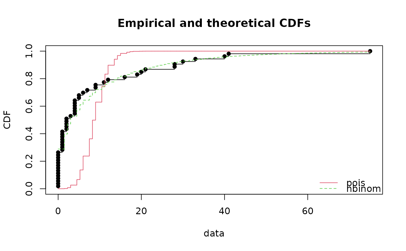
# (5) fit discrete distributions (Poisson and negative binomial)
#
data(toxocara)
number <- toxocara$number
fitp <- fitdist(number,"pois")
summary(fitp)
#> Fitting of the distribution ' pois ' by maximum likelihood
#> Parameters :
#> estimate Std. Error
#> lambda 8.679245 0.4046719
#> Loglikelihood: -507.5334 AIC: 1017.067 BIC: 1019.037
plot(fitp)
gofstat(list(fitW, fitg, fitln), fitnames=c("Weibull", "gamma", "lognormal"))
#> Goodness-of-fit statistics
#> Weibull gamma lognormal
#> Kolmogorov-Smirnov statistic 0.1396646 0.1281486 0.1493090
#> Cramer-von Mises statistic 0.6840994 0.6936274 0.8277358
#> Anderson-Darling statistic 3.5736460 3.5672625 4.5436542
#>
#> Goodness-of-fit criteria
#> Weibull gamma lognormal
#> Akaike's Information Criterion 2514.449 2511.250 2526.639
#> Bayesian Information Criterion 2521.524 2518.325 2533.713
# (4) defining your own distribution functions, here for the Gumbel distribution
# for other distributions, see the CRAN task view
# dedicated to probability distributions
#
dgumbel <- function(x, a, b) 1/b*exp((a-x)/b)*exp(-exp((a-x)/b))
pgumbel <- function(q, a, b) exp(-exp((a-q)/b))
qgumbel <- function(p, a, b) a-b*log(-log(p))
fitgumbel <- fitdist(serving, "gumbel", start=list(a=10, b=10))
#> Error in fitdist(serving, "gumbel", start = list(a = 10, b = 10)): Your <distr> argument should be either a character string or a function so that d<distr> exists.Otherwise please wrap it in another function with that name.
summary(fitgumbel)
#> Error: object 'fitgumbel' not found
plot(fitgumbel)
#> Error: object 'fitgumbel' not found
# (5) fit discrete distributions (Poisson and negative binomial)
#
data(toxocara)
number <- toxocara$number
fitp <- fitdist(number,"pois")
summary(fitp)
#> Fitting of the distribution ' pois ' by maximum likelihood
#> Parameters :
#> estimate Std. Error
#> lambda 8.679245 0.4046719
#> Loglikelihood: -507.5334 AIC: 1017.067 BIC: 1019.037
plot(fitp)
 fitnb <- fitdist(number,"nbinom")
summary(fitnb)
#> Fitting of the distribution ' nbinom ' by maximum likelihood
#> Parameters :
#> estimate Std. Error
#> size 0.3971457 0.08289027
#> mu 8.6802520 1.93501002
#> Loglikelihood: -159.3441 AIC: 322.6882 BIC: 326.6288
#> Correlation matrix:
#> size mu
#> size 1.000000000 -0.000103854
#> mu -0.000103854 1.000000000
#>
plot(fitnb)
fitnb <- fitdist(number,"nbinom")
summary(fitnb)
#> Fitting of the distribution ' nbinom ' by maximum likelihood
#> Parameters :
#> estimate Std. Error
#> size 0.3971457 0.08289027
#> mu 8.6802520 1.93501002
#> Loglikelihood: -159.3441 AIC: 322.6882 BIC: 326.6288
#> Correlation matrix:
#> size mu
#> size 1.000000000 -0.000103854
#> mu -0.000103854 1.000000000
#>
plot(fitnb)
 cdfcomp(list(fitp,fitnb))
 gofstat(list(fitp,fitnb))
#> Chi-squared statistic: 31256.96 7.48606
#> Degree of freedom of the Chi-squared distribution: 5 4
#> Chi-squared p-value: 0 0.1123255
#> the p-value may be wrong with some theoretical counts < 5
#> Chi-squared table:
#> obscounts theo 1-mle-pois theo 2-mle-nbinom
#> <= 0 14 0.009014207 15.295027
#> <= 1 8 0.078236515 5.808596
#> <= 3 6 1.321767253 6.845015
#> <= 4 6 2.131297825 2.407815
#> <= 9 6 29.827829425 7.835196
#> <= 21 6 19.626223437 8.271110
#> > 21 7 0.005631338 6.537242
#>
#> Goodness-of-fit criteria
#> 1-mle-pois 2-mle-nbinom
#> Akaike's Information Criterion 1017.067 322.6882
#> Bayesian Information Criterion 1019.037 326.6288
# (6) how to change the optimisation method?
#
data(groundbeef)
serving <- groundbeef$serving
fitdist(serving, "gamma", optim.method="Nelder-Mead")
#> Fitting of the distribution ' gamma ' by maximum likelihood
#> Parameters:
#> estimate Std. Error
#> shape 4.00955898 0.341451640
#> rate 0.05443907 0.004937239
fitdist(serving, "gamma", optim.method="BFGS")
#> Fitting of the distribution ' gamma ' by maximum likelihood
#> Parameters:
#> estimate Std. Error
#> shape 4.21183650 0.359345675
#> rate 0.05719298 0.005180917
fitdist(serving, "gamma", optim.method="SANN")
#> Fitting of the distribution ' gamma ' by maximum likelihood
#> Parameters:
#> estimate Std. Error
#> shape 4.21183859 0.359345812
#> rate 0.05719058 0.005180698
# (7) custom optimization function
#
# \donttest{
#create the sample
mysample <- rexp(100, 5)
mystart <- list(rate=8)
res1 <- fitdist(mysample, dexp, start= mystart, optim.method="Nelder-Mead")
#show the result
summary(res1)
#> Fitting of the distribution ' exp ' by maximum likelihood
#> Parameters :
#> estimate Std. Error
#> rate 4.785937 0.4785937
#> Loglikelihood: 56.57608 AIC: -111.1522 BIC: -108.547
#the warning tell us to use optimise, because the Nelder-Mead is not adequate.
#to meet the standard 'fn' argument and specific name arguments, we wrap optimize,
myoptimize <- function(fn, par, ...)
{
res <- optimize(f=fn, ..., maximum=FALSE)
#assume the optimization function minimize
standardres <- c(res, convergence=0, value=res$objective,
par=res$minimum, hessian=NA)
return(standardres)
}
#call fitdist with a 'custom' optimization function
res2 <- fitdist(mysample, "exp", start=mystart, custom.optim=myoptimize,
interval=c(0, 100))
#show the result
summary(res2)
#> Fitting of the distribution ' exp ' by maximum likelihood
#> Parameters :
#> estimate
#> rate 4.786311
#> Loglikelihood: 56.57608 AIC: -111.1522 BIC: -108.547
# }
# (8) custom optimization function - another example with the genetic algorithm
#
# \donttest{
#set a sample
fit1 <- fitdist(serving, "gamma")
summary(fit1)
#> Fitting of the distribution ' gamma ' by maximum likelihood
#> Parameters :
#> estimate Std. Error
#> shape 4.00955898 0.341451640
#> rate 0.05443907 0.004937239
#> Loglikelihood: -1253.625 AIC: 2511.25 BIC: 2518.325
#> Correlation matrix:
#> shape rate
#> shape 1.0000000 0.9384578
#> rate 0.9384578 1.0000000
#>
#wrap genoud function rgenoud package
mygenoud <- function(fn, par, ...)
{
require("rgenoud")
res <- genoud(fn, starting.values=par, ...)
standardres <- c(res, convergence=0)
return(standardres)
}
#call fitdist with a 'custom' optimization function
fit2 <- fitdist(serving, "gamma", custom.optim=mygenoud, nvars=2,
Domains=cbind(c(0, 0), c(10, 10)), boundary.enforcement=1,
print.level=1, hessian=TRUE)
#> Loading required package: rgenoud
#> ## rgenoud (Version 5.9-0.11, Build Date: 2024-10-03)
#> ## See http://sekhon.berkeley.edu/rgenoud for additional documentation.
#> ## Please cite software as:
#> ## Walter Mebane, Jr. and Jasjeet S. Sekhon. 2011.
#> ## ``Genetic Optimization Using Derivatives: The rgenoud package for R.''
#> ## Journal of Statistical Software, 42(11): 1-26.
#> ##
#>
#>
#> Tue Jun 30 14:50:58 2026
#> Domains:
#> 0.000000e+00 <= X1 <= 1.000000e+01
#> 0.000000e+00 <= X2 <= 1.000000e+01
#>
#> Data Type: Floating Point
#> Operators (code number, name, population)
#> (1) Cloning........................... 122
#> (2) Uniform Mutation.................. 125
#> (3) Boundary Mutation................. 125
#> (4) Non-Uniform Mutation.............. 125
#> (5) Polytope Crossover................ 125
#> (6) Simple Crossover.................. 126
#> (7) Whole Non-Uniform Mutation........ 125
#> (8) Heuristic Crossover............... 126
#> (9) Local-Minimum Crossover........... 0
#>
#> HARD Maximum Number of Generations: 100
#> Maximum Nonchanging Generations: 10
#> Population size : 1000
#> Convergence Tolerance: 1.000000e-03
#>
#> Using the BFGS Derivative Based Optimizer on the Best Individual Each Generation.
#> Checking Gradients before Stopping.
#> Not Using Out of Bounds Individuals But Allowing Trespassing.
#>
#> Minimization Problem.
#>
#>
#> Generation# Solution Value
#>
#> 0 4.936206e+00
#>
#> 'wait.generations' limit reached.
#> No significant improvement in 10 generations.
#>
#> Solution Fitness Value: 4.935532e+00
#>
#> Parameters at the Solution (parameter, gradient):
#>
#> X[ 1] : 4.008339e+00 G[ 1] : -7.615302e-09
#> X[ 2] : 5.442735e-02 G[ 2] : 3.076197e-07
#>
#> Solution Found Generation 1
#> Number of Generations Run 11
#>
#> Tue Jun 30 14:50:59 2026
#> Total run time : 0 hours 0 minutes and 1 seconds
summary(fit2)
#> Fitting of the distribution ' gamma ' by maximum likelihood
#> Parameters :
#> estimate Std. Error
#> shape 4.00833894 0.341343832
#> rate 0.05442735 0.004936215
#> Loglikelihood: -1253.625 AIC: 2511.25 BIC: 2518.325
#> Correlation matrix:
#> shape rate
#> shape 1.0000000 0.9384394
#> rate 0.9384394 1.0000000
#>
# }
# (9) estimation of the standard deviation of a gamma distribution
# by maximum likelihood with the shape fixed at 4 using the argument fix.arg
#
data(groundbeef)
serving <- groundbeef$serving
f1c <- fitdist(serving,"gamma",start=list(rate=0.1),fix.arg=list(shape=4))
summary(f1c)
#> Fitting of the distribution ' gamma ' by maximum likelihood
#> Parameters :
#> estimate Std. Error
#> rate 0.05431619 0.001703472
#> Fixed parameters:
#> value
#> shape 4
#> Loglikelihood: -1253.625 AIC: 2509.251 BIC: 2512.788
plot(f1c)
gofstat(list(fitp,fitnb))
#> Chi-squared statistic: 31256.96 7.48606
#> Degree of freedom of the Chi-squared distribution: 5 4
#> Chi-squared p-value: 0 0.1123255
#> the p-value may be wrong with some theoretical counts < 5
#> Chi-squared table:
#> obscounts theo 1-mle-pois theo 2-mle-nbinom
#> <= 0 14 0.009014207 15.295027
#> <= 1 8 0.078236515 5.808596
#> <= 3 6 1.321767253 6.845015
#> <= 4 6 2.131297825 2.407815
#> <= 9 6 29.827829425 7.835196
#> <= 21 6 19.626223437 8.271110
#> > 21 7 0.005631338 6.537242
#>
#> Goodness-of-fit criteria
#> 1-mle-pois 2-mle-nbinom
#> Akaike's Information Criterion 1017.067 322.6882
#> Bayesian Information Criterion 1019.037 326.6288
# (6) how to change the optimisation method?
#
data(groundbeef)
serving <- groundbeef$serving
fitdist(serving, "gamma", optim.method="Nelder-Mead")
#> Fitting of the distribution ' gamma ' by maximum likelihood
#> Parameters:
#> estimate Std. Error
#> shape 4.00955898 0.341451640
#> rate 0.05443907 0.004937239
fitdist(serving, "gamma", optim.method="BFGS")
#> Fitting of the distribution ' gamma ' by maximum likelihood
#> Parameters:
#> estimate Std. Error
#> shape 4.21183650 0.359345675
#> rate 0.05719298 0.005180917
fitdist(serving, "gamma", optim.method="SANN")
#> Fitting of the distribution ' gamma ' by maximum likelihood
#> Parameters:
#> estimate Std. Error
#> shape 4.21183859 0.359345812
#> rate 0.05719058 0.005180698
# (7) custom optimization function
#
# \donttest{
#create the sample
mysample <- rexp(100, 5)
mystart <- list(rate=8)
res1 <- fitdist(mysample, dexp, start= mystart, optim.method="Nelder-Mead")
#show the result
summary(res1)
#> Fitting of the distribution ' exp ' by maximum likelihood
#> Parameters :
#> estimate Std. Error
#> rate 4.785937 0.4785937
#> Loglikelihood: 56.57608 AIC: -111.1522 BIC: -108.547
#the warning tell us to use optimise, because the Nelder-Mead is not adequate.
#to meet the standard 'fn' argument and specific name arguments, we wrap optimize,
myoptimize <- function(fn, par, ...)
{
res <- optimize(f=fn, ..., maximum=FALSE)
#assume the optimization function minimize
standardres <- c(res, convergence=0, value=res$objective,
par=res$minimum, hessian=NA)
return(standardres)
}
#call fitdist with a 'custom' optimization function
res2 <- fitdist(mysample, "exp", start=mystart, custom.optim=myoptimize,
interval=c(0, 100))
#show the result
summary(res2)
#> Fitting of the distribution ' exp ' by maximum likelihood
#> Parameters :
#> estimate
#> rate 4.786311
#> Loglikelihood: 56.57608 AIC: -111.1522 BIC: -108.547
# }
# (8) custom optimization function - another example with the genetic algorithm
#
# \donttest{
#set a sample
fit1 <- fitdist(serving, "gamma")
summary(fit1)
#> Fitting of the distribution ' gamma ' by maximum likelihood
#> Parameters :
#> estimate Std. Error
#> shape 4.00955898 0.341451640
#> rate 0.05443907 0.004937239
#> Loglikelihood: -1253.625 AIC: 2511.25 BIC: 2518.325
#> Correlation matrix:
#> shape rate
#> shape 1.0000000 0.9384578
#> rate 0.9384578 1.0000000
#>
#wrap genoud function rgenoud package
mygenoud <- function(fn, par, ...)
{
require("rgenoud")
res <- genoud(fn, starting.values=par, ...)
standardres <- c(res, convergence=0)
return(standardres)
}
#call fitdist with a 'custom' optimization function
fit2 <- fitdist(serving, "gamma", custom.optim=mygenoud, nvars=2,
Domains=cbind(c(0, 0), c(10, 10)), boundary.enforcement=1,
print.level=1, hessian=TRUE)
#> Loading required package: rgenoud
#> ## rgenoud (Version 5.9-0.11, Build Date: 2024-10-03)
#> ## See http://sekhon.berkeley.edu/rgenoud for additional documentation.
#> ## Please cite software as:
#> ## Walter Mebane, Jr. and Jasjeet S. Sekhon. 2011.
#> ## ``Genetic Optimization Using Derivatives: The rgenoud package for R.''
#> ## Journal of Statistical Software, 42(11): 1-26.
#> ##
#>
#>
#> Tue Jun 30 14:50:58 2026
#> Domains:
#> 0.000000e+00 <= X1 <= 1.000000e+01
#> 0.000000e+00 <= X2 <= 1.000000e+01
#>
#> Data Type: Floating Point
#> Operators (code number, name, population)
#> (1) Cloning........................... 122
#> (2) Uniform Mutation.................. 125
#> (3) Boundary Mutation................. 125
#> (4) Non-Uniform Mutation.............. 125
#> (5) Polytope Crossover................ 125
#> (6) Simple Crossover.................. 126
#> (7) Whole Non-Uniform Mutation........ 125
#> (8) Heuristic Crossover............... 126
#> (9) Local-Minimum Crossover........... 0
#>
#> HARD Maximum Number of Generations: 100
#> Maximum Nonchanging Generations: 10
#> Population size : 1000
#> Convergence Tolerance: 1.000000e-03
#>
#> Using the BFGS Derivative Based Optimizer on the Best Individual Each Generation.
#> Checking Gradients before Stopping.
#> Not Using Out of Bounds Individuals But Allowing Trespassing.
#>
#> Minimization Problem.
#>
#>
#> Generation# Solution Value
#>
#> 0 4.936206e+00
#>
#> 'wait.generations' limit reached.
#> No significant improvement in 10 generations.
#>
#> Solution Fitness Value: 4.935532e+00
#>
#> Parameters at the Solution (parameter, gradient):
#>
#> X[ 1] : 4.008339e+00 G[ 1] : -7.615302e-09
#> X[ 2] : 5.442735e-02 G[ 2] : 3.076197e-07
#>
#> Solution Found Generation 1
#> Number of Generations Run 11
#>
#> Tue Jun 30 14:50:59 2026
#> Total run time : 0 hours 0 minutes and 1 seconds
summary(fit2)
#> Fitting of the distribution ' gamma ' by maximum likelihood
#> Parameters :
#> estimate Std. Error
#> shape 4.00833894 0.341343832
#> rate 0.05442735 0.004936215
#> Loglikelihood: -1253.625 AIC: 2511.25 BIC: 2518.325
#> Correlation matrix:
#> shape rate
#> shape 1.0000000 0.9384394
#> rate 0.9384394 1.0000000
#>
# }
# (9) estimation of the standard deviation of a gamma distribution
# by maximum likelihood with the shape fixed at 4 using the argument fix.arg
#
data(groundbeef)
serving <- groundbeef$serving
f1c <- fitdist(serving,"gamma",start=list(rate=0.1),fix.arg=list(shape=4))
summary(f1c)
#> Fitting of the distribution ' gamma ' by maximum likelihood
#> Parameters :
#> estimate Std. Error
#> rate 0.05431619 0.001703472
#> Fixed parameters:
#> value
#> shape 4
#> Loglikelihood: -1253.625 AIC: 2509.251 BIC: 2512.788
plot(f1c)
 # (10) fit of a Weibull distribution to serving size data
# by maximum likelihood estimation
# or by quantile matching estimation (in this example
# matching first and third quartiles)
#
data(groundbeef)
serving <- groundbeef$serving
fWmle <- fitdist(serving, "weibull")
summary(fWmle)
#> Fitting of the distribution ' weibull ' by maximum likelihood
#> Parameters :
#> estimate Std. Error
#> shape 2.185885 0.1045755
#> scale 83.347679 2.5268631
#> Loglikelihood: -1255.225 AIC: 2514.449 BIC: 2521.524
#> Correlation matrix:
#> shape scale
#> shape 1.000000 0.321821
#> scale 0.321821 1.000000
#>
plot(fWmle)
# (10) fit of a Weibull distribution to serving size data
# by maximum likelihood estimation
# or by quantile matching estimation (in this example
# matching first and third quartiles)
#
data(groundbeef)
serving <- groundbeef$serving
fWmle <- fitdist(serving, "weibull")
summary(fWmle)
#> Fitting of the distribution ' weibull ' by maximum likelihood
#> Parameters :
#> estimate Std. Error
#> shape 2.185885 0.1045755
#> scale 83.347679 2.5268631
#> Loglikelihood: -1255.225 AIC: 2514.449 BIC: 2521.524
#> Correlation matrix:
#> shape scale
#> shape 1.000000 0.321821
#> scale 0.321821 1.000000
#>
plot(fWmle)
 gofstat(fWmle)
#> Goodness-of-fit statistics
#> 1-mle-weibull
#> Kolmogorov-Smirnov statistic 0.1396646
#> Cramer-von Mises statistic 0.6840994
#> Anderson-Darling statistic 3.5736460
#>
#> Goodness-of-fit criteria
#> 1-mle-weibull
#> Akaike's Information Criterion 2514.449
#> Bayesian Information Criterion 2521.524
fWqme <- fitdist(serving, "weibull", method="qme", probs=c(0.25, 0.75))
summary(fWqme)
#> Fitting of the distribution ' weibull ' by matching quantiles
#> Parameters :
#> estimate
#> shape 2.268699
#> scale 86.590853
#> Loglikelihood: -1256.129 AIC: 2516.258 BIC: 2523.332
plot(fWqme)
gofstat(fWmle)
#> Goodness-of-fit statistics
#> 1-mle-weibull
#> Kolmogorov-Smirnov statistic 0.1396646
#> Cramer-von Mises statistic 0.6840994
#> Anderson-Darling statistic 3.5736460
#>
#> Goodness-of-fit criteria
#> 1-mle-weibull
#> Akaike's Information Criterion 2514.449
#> Bayesian Information Criterion 2521.524
fWqme <- fitdist(serving, "weibull", method="qme", probs=c(0.25, 0.75))
summary(fWqme)
#> Fitting of the distribution ' weibull ' by matching quantiles
#> Parameters :
#> estimate
#> shape 2.268699
#> scale 86.590853
#> Loglikelihood: -1256.129 AIC: 2516.258 BIC: 2523.332
plot(fWqme)
 gofstat(fWqme)
#> Goodness-of-fit statistics
#> 1-qme-weibull
#> Kolmogorov-Smirnov statistic 0.1692858
#> Cramer-von Mises statistic 0.9664709
#> Anderson-Darling statistic 4.8479858
#>
#> Goodness-of-fit criteria
#> 1-qme-weibull
#> Akaike's Information Criterion 2516.258
#> Bayesian Information Criterion 2523.332
# (11) Fit of a Pareto distribution by numerical moment matching estimation
#
# \donttest{
require("actuar")
#> Loading required package: actuar
#>
#> Attaching package: ‘actuar’
#> The following objects are masked from ‘package:stats’:
#>
#> sd, var
#> The following object is masked from ‘package:grDevices’:
#>
#> cm
#simulate a sample
x4 <- rpareto(1000, 6, 2)
#empirical raw moment
memp <- function(x, order) mean(x^order)
#fit
fP <- fitdist(x4, "pareto", method="mme", order=c(1, 2), memp="memp",
start=list(shape=10, scale=10), lower=1, upper=Inf)
#> Error in mmedist(data, distname, start = arg_startfix$start.arg, fix.arg = arg_startfix$fix.arg, checkstartfix = TRUE, calcvcov = calcvcov, ...): the empirical moment must be defined as a function
summary(fP)
#> Error: object 'fP' not found
plot(fP)
#> Error: object 'fP' not found
# }
# (12) Fit of a Weibull distribution to serving size data by maximum
# goodness-of-fit estimation using all the distances available
#
# \donttest{
data(groundbeef)
serving <- groundbeef$serving
(f1 <- fitdist(serving, "weibull", method="mge", gof="CvM"))
#> Fitting of the distribution ' weibull ' by maximum goodness-of-fit
#> Parameters:
#> estimate
#> shape 2.093204
#> scale 82.660014
(f2 <- fitdist(serving, "weibull", method="mge", gof="KS"))
#> Fitting of the distribution ' weibull ' by maximum goodness-of-fit
#> Parameters:
#> estimate
#> shape 2.065634
#> scale 81.450487
(f3 <- fitdist(serving, "weibull", method="mge", gof="AD"))
#> Fitting of the distribution ' weibull ' by maximum goodness-of-fit
#> Parameters:
#> estimate
#> shape 2.125425
#> scale 82.890502
(f4 <- fitdist(serving, "weibull", method="mge", gof="ADR"))
#> Fitting of the distribution ' weibull ' by maximum goodness-of-fit
#> Parameters:
#> estimate
#> shape 2.072035
#> scale 82.762593
(f5 <- fitdist(serving, "weibull", method="mge", gof="ADL"))
#> Fitting of the distribution ' weibull ' by maximum goodness-of-fit
#> Parameters:
#> estimate
#> shape 2.197498
#> scale 82.016005
(f6 <- fitdist(serving, "weibull", method="mge", gof="AD2R"))
#> Fitting of the distribution ' weibull ' by maximum goodness-of-fit
#> Parameters:
#> estimate
#> shape 1.90328
#> scale 81.33464
(f7 <- fitdist(serving, "weibull", method="mge", gof="AD2L"))
#> Fitting of the distribution ' weibull ' by maximum goodness-of-fit
#> Parameters:
#> estimate
#> shape 2.483836
#> scale 78.252113
(f8 <- fitdist(serving, "weibull", method="mge", gof="AD2"))
#> Fitting of the distribution ' weibull ' by maximum goodness-of-fit
#> Parameters:
#> estimate
#> shape 2.081168
#> scale 85.281194
cdfcomp(list(f1, f2, f3, f4, f5, f6, f7, f8))
gofstat(fWqme)
#> Goodness-of-fit statistics
#> 1-qme-weibull
#> Kolmogorov-Smirnov statistic 0.1692858
#> Cramer-von Mises statistic 0.9664709
#> Anderson-Darling statistic 4.8479858
#>
#> Goodness-of-fit criteria
#> 1-qme-weibull
#> Akaike's Information Criterion 2516.258
#> Bayesian Information Criterion 2523.332
# (11) Fit of a Pareto distribution by numerical moment matching estimation
#
# \donttest{
require("actuar")
#> Loading required package: actuar
#>
#> Attaching package: ‘actuar’
#> The following objects are masked from ‘package:stats’:
#>
#> sd, var
#> The following object is masked from ‘package:grDevices’:
#>
#> cm
#simulate a sample
x4 <- rpareto(1000, 6, 2)
#empirical raw moment
memp <- function(x, order) mean(x^order)
#fit
fP <- fitdist(x4, "pareto", method="mme", order=c(1, 2), memp="memp",
start=list(shape=10, scale=10), lower=1, upper=Inf)
#> Error in mmedist(data, distname, start = arg_startfix$start.arg, fix.arg = arg_startfix$fix.arg, checkstartfix = TRUE, calcvcov = calcvcov, ...): the empirical moment must be defined as a function
summary(fP)
#> Error: object 'fP' not found
plot(fP)
#> Error: object 'fP' not found
# }
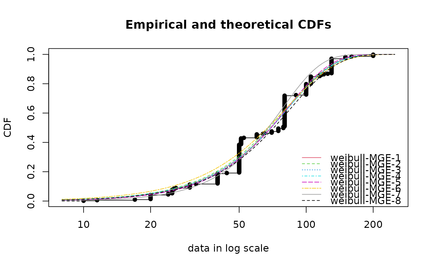
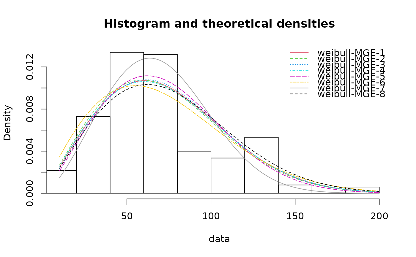
# (12) Fit of a Weibull distribution to serving size data by maximum
# goodness-of-fit estimation using all the distances available
#
# \donttest{
data(groundbeef)
serving <- groundbeef$serving
(f1 <- fitdist(serving, "weibull", method="mge", gof="CvM"))
#> Fitting of the distribution ' weibull ' by maximum goodness-of-fit
#> Parameters:
#> estimate
#> shape 2.093204
#> scale 82.660014
(f2 <- fitdist(serving, "weibull", method="mge", gof="KS"))
#> Fitting of the distribution ' weibull ' by maximum goodness-of-fit
#> Parameters:
#> estimate
#> shape 2.065634
#> scale 81.450487
(f3 <- fitdist(serving, "weibull", method="mge", gof="AD"))
#> Fitting of the distribution ' weibull ' by maximum goodness-of-fit
#> Parameters:
#> estimate
#> shape 2.125425
#> scale 82.890502
(f4 <- fitdist(serving, "weibull", method="mge", gof="ADR"))
#> Fitting of the distribution ' weibull ' by maximum goodness-of-fit
#> Parameters:
#> estimate
#> shape 2.072035
#> scale 82.762593
(f5 <- fitdist(serving, "weibull", method="mge", gof="ADL"))
#> Fitting of the distribution ' weibull ' by maximum goodness-of-fit
#> Parameters:
#> estimate
#> shape 2.197498
#> scale 82.016005
(f6 <- fitdist(serving, "weibull", method="mge", gof="AD2R"))
#> Fitting of the distribution ' weibull ' by maximum goodness-of-fit
#> Parameters:
#> estimate
#> shape 1.90328
#> scale 81.33464
(f7 <- fitdist(serving, "weibull", method="mge", gof="AD2L"))
#> Fitting of the distribution ' weibull ' by maximum goodness-of-fit
#> Parameters:
#> estimate
#> shape 2.483836
#> scale 78.252113
(f8 <- fitdist(serving, "weibull", method="mge", gof="AD2"))
#> Fitting of the distribution ' weibull ' by maximum goodness-of-fit
#> Parameters:
#> estimate
#> shape 2.081168
#> scale 85.281194
cdfcomp(list(f1, f2, f3, f4, f5, f6, f7, f8))
 cdfcomp(list(f1, f2, f3, f4, f5, f6, f7, f8),
xlogscale=TRUE, xlim=c(8, 250), verticals=TRUE)
cdfcomp(list(f1, f2, f3, f4, f5, f6, f7, f8),
xlogscale=TRUE, xlim=c(8, 250), verticals=TRUE)
 denscomp(list(f1, f2, f3, f4, f5, f6, f7, f8))
 # }
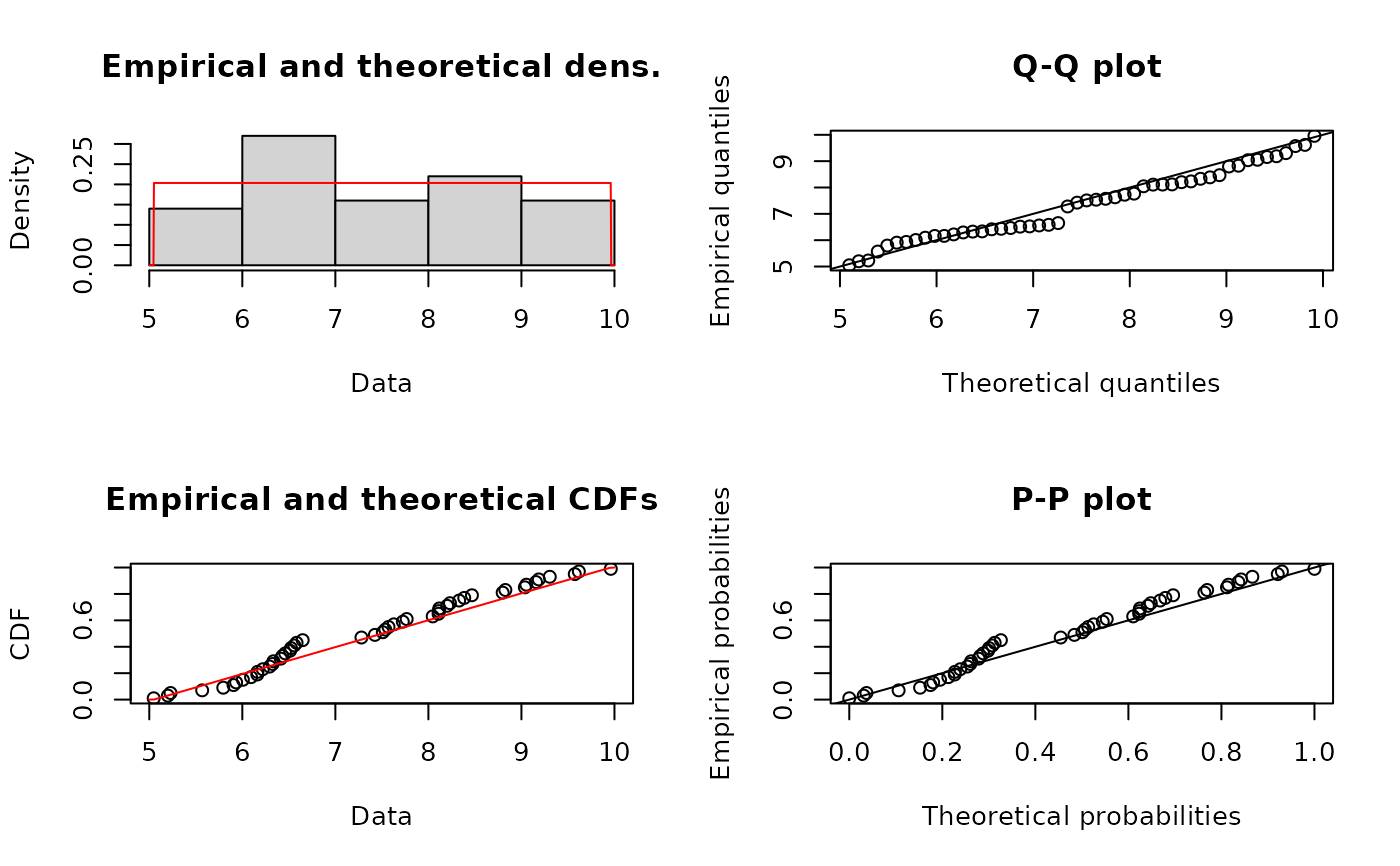
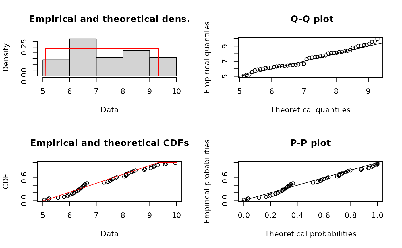
# (13) Fit of a uniform distribution using maximum likelihood
# (a closed formula is used in this special case where the loglikelihood is not defined),
# or maximum goodness-of-fit with Cramer-von Mises or Kolmogorov-Smirnov distance
#
u <- runif(50, min=5, max=10)
fumle <- fitdist(u, "unif", method="mle")
summary(fumle)
#> Fitting of the distribution ' unif ' by maximum likelihood
#> Parameters :
#> estimate
#> min 5.100788
#> max 9.925639
#> Loglikelihood: -78.689 AIC: 161.378 BIC: 165.202
plot(fumle)
# }
# (13) Fit of a uniform distribution using maximum likelihood
# (a closed formula is used in this special case where the loglikelihood is not defined),
# or maximum goodness-of-fit with Cramer-von Mises or Kolmogorov-Smirnov distance
#
u <- runif(50, min=5, max=10)
fumle <- fitdist(u, "unif", method="mle")
summary(fumle)
#> Fitting of the distribution ' unif ' by maximum likelihood
#> Parameters :
#> estimate
#> min 5.100788
#> max 9.925639
#> Loglikelihood: -78.689 AIC: 161.378 BIC: 165.202
plot(fumle)
 gofstat(fumle)
#> Goodness-of-fit statistics
#> 1-mle-unif
#> Kolmogorov-Smirnov statistic 0.1314321
#> Cramer-von Mises statistic 0.1726303
#> Anderson-Darling statistic Inf
#>
#> Goodness-of-fit criteria
#> 1-mle-unif
#> Akaike's Information Criterion 161.378
#> Bayesian Information Criterion 165.202
fuCvM <- fitdist(u, "unif", method="mge", gof="CvM")
summary(fuCvM)
#> Fitting of the distribution ' unif ' by maximum goodness-of-fit
#> Parameters :
#> estimate
#> min 5.357159
#> max 10.103398
#> Loglikelihood: -Inf AIC: Inf BIC: Inf
plot(fuCvM)
gofstat(fumle)
#> Goodness-of-fit statistics
#> 1-mle-unif
#> Kolmogorov-Smirnov statistic 0.1314321
#> Cramer-von Mises statistic 0.1726303
#> Anderson-Darling statistic Inf
#>
#> Goodness-of-fit criteria
#> 1-mle-unif
#> Akaike's Information Criterion 161.378
#> Bayesian Information Criterion 165.202
fuCvM <- fitdist(u, "unif", method="mge", gof="CvM")
summary(fuCvM)
#> Fitting of the distribution ' unif ' by maximum goodness-of-fit
#> Parameters :
#> estimate
#> min 5.357159
#> max 10.103398
#> Loglikelihood: -Inf AIC: Inf BIC: Inf
plot(fuCvM)
 gofstat(fuCvM)
#> Goodness-of-fit statistics
#> 1-mge-unif
#> Kolmogorov-Smirnov statistic 0.08703740
#> Cramer-von Mises statistic 0.08128704
#> Anderson-Darling statistic Inf
#>
#> Goodness-of-fit criteria
#> 1-mge-unif
#> Akaike's Information Criterion Inf
#> Bayesian Information Criterion Inf
fuKS <- fitdist(u, "unif", method="mge", gof="KS")
summary(fuKS)
#> Fitting of the distribution ' unif ' by maximum goodness-of-fit
#> Parameters :
#> estimate
#> min 5.386917
#> max 10.141086
#> Loglikelihood: -Inf AIC: Inf BIC: Inf
plot(fuKS)
gofstat(fuCvM)
#> Goodness-of-fit statistics
#> 1-mge-unif
#> Kolmogorov-Smirnov statistic 0.08703740
#> Cramer-von Mises statistic 0.08128704
#> Anderson-Darling statistic Inf
#>
#> Goodness-of-fit criteria
#> 1-mge-unif
#> Akaike's Information Criterion Inf
#> Bayesian Information Criterion Inf
fuKS <- fitdist(u, "unif", method="mge", gof="KS")
summary(fuKS)
#> Fitting of the distribution ' unif ' by maximum goodness-of-fit
#> Parameters :
#> estimate
#> min 5.386917
#> max 10.141086
#> Loglikelihood: -Inf AIC: Inf BIC: Inf
plot(fuKS)
 gofstat(fuKS)
#> Goodness-of-fit statistics
#> 1-mge-unif
#> Kolmogorov-Smirnov statistic 0.07986562
#> Cramer-von Mises statistic 0.08369415
#> Anderson-Darling statistic Inf
#>
#> Goodness-of-fit criteria
#> 1-mge-unif
#> Akaike's Information Criterion Inf
#> Bayesian Information Criterion Inf
# (14) scaling problem
# the simulated dataset (below) has particularly small values, hence without scaling (10^0),
# the optimization raises an error. The for loop shows how scaling by 10^i
# for i=1,...,6 makes the fitting procedure work correctly.
x2 <- rnorm(100, 1e-4, 2e-4)
for(i in 0:6)
cat(i, try(fitdist(x2*10^i, "cauchy", method="mle")$estimate, silent=TRUE), "\n")
#> <simpleError in optim(par = vstart, fn = fnobj, fix.arg = fix.arg, obs = data, gr = gradient, ddistnam = ddistname, hessian = TRUE, method = meth, lower = lower, upper = upper, ...): non-finite finite-difference value [2]>
#> 0 Error in fitdist(x2 * 10^i, "cauchy", method = "mle") :
#> the function mle failed to estimate the parameters,
#> with the error code 100
#>
#>
#> <simpleError in optim(par = vstart, fn = fnobj, fix.arg = fix.arg, obs = data, gr = gradient, ddistnam = ddistname, hessian = TRUE, method = meth, lower = lower, upper = upper, ...): non-finite finite-difference value [2]>
#> 1 Error in fitdist(x2 * 10^i, "cauchy", method = "mle") :
#> the function mle failed to estimate the parameters,
#> with the error code 100
#>
#>
#> 2 0.008532115 0.01042502
#> 3 0.08531779 0.1042657
#> 4 0.8532115 1.042502
#> 5 8.531511 10.42933
#> 6 85.31511 104.2933
# (15) Fit of a normal distribution on acute toxicity values of endosulfan in log10 for
# nonarthropod invertebrates, using maximum likelihood estimation
# to estimate what is called a species sensitivity distribution
# (SSD) in ecotoxicology, followed by estimation of the 5 percent quantile value of
# the fitted distribution (which is called the 5 percent hazardous concentration, HC5,
# in ecotoxicology) and estimation of other quantiles.
#
data(endosulfan)
ATV <- subset(endosulfan, group == "NonArthroInvert")$ATV
log10ATV <- log10(subset(endosulfan, group == "NonArthroInvert")$ATV)
fln <- fitdist(log10ATV, "norm")
quantile(fln, probs = 0.05)
#> Estimated quantiles for each specified probability (non-censored data)
#> p=0.05
#> estimate 1.744227
quantile(fln, probs = c(0.05, 0.1, 0.2))
#> Estimated quantiles for each specified probability (non-censored data)
#> p=0.05 p=0.1 p=0.2
#> estimate 1.744227 2.080093 2.4868
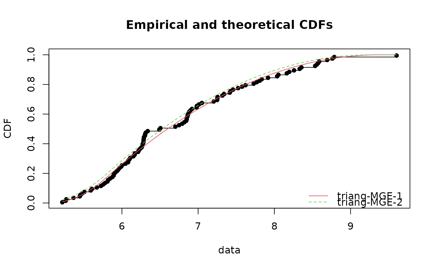
# (16) Fit of a triangular distribution using Cramer-von Mises or
# Kolmogorov-Smirnov distance
#
# \donttest{
require("mc2d")
#> Loading required package: mc2d
#> Loading required package: mvtnorm
#>
#> Attaching package: ‘mc2d’
#> The following objects are masked from ‘package:base’:
#>
#> pmax, pmin
t <- rtriang(100, min=5, mode=6, max=10)
fCvM <- fitdist(t, "triang", method="mge", start = list(min=4, mode=6,max=9), gof="CvM")
#> Warning: Some parameter names have no starting/fixed value but have a default value: mean.
fKS <- fitdist(t, "triang", method="mge", start = list(min=4, mode=6,max=9), gof="KS")
#> Warning: Some parameter names have no starting/fixed value but have a default value: mean.
cdfcomp(list(fCvM,fKS))
gofstat(fuKS)
#> Goodness-of-fit statistics
#> 1-mge-unif
#> Kolmogorov-Smirnov statistic 0.07986562
#> Cramer-von Mises statistic 0.08369415
#> Anderson-Darling statistic Inf
#>
#> Goodness-of-fit criteria
#> 1-mge-unif
#> Akaike's Information Criterion Inf
#> Bayesian Information Criterion Inf
# (14) scaling problem
# the simulated dataset (below) has particularly small values, hence without scaling (10^0),
# the optimization raises an error. The for loop shows how scaling by 10^i
# for i=1,...,6 makes the fitting procedure work correctly.
x2 <- rnorm(100, 1e-4, 2e-4)
for(i in 0:6)
cat(i, try(fitdist(x2*10^i, "cauchy", method="mle")$estimate, silent=TRUE), "\n")
#> <simpleError in optim(par = vstart, fn = fnobj, fix.arg = fix.arg, obs = data, gr = gradient, ddistnam = ddistname, hessian = TRUE, method = meth, lower = lower, upper = upper, ...): non-finite finite-difference value [2]>
#> 0 Error in fitdist(x2 * 10^i, "cauchy", method = "mle") :
#> the function mle failed to estimate the parameters,
#> with the error code 100
#>
#>
#> <simpleError in optim(par = vstart, fn = fnobj, fix.arg = fix.arg, obs = data, gr = gradient, ddistnam = ddistname, hessian = TRUE, method = meth, lower = lower, upper = upper, ...): non-finite finite-difference value [2]>
#> 1 Error in fitdist(x2 * 10^i, "cauchy", method = "mle") :
#> the function mle failed to estimate the parameters,
#> with the error code 100
#>
#>
#> 2 0.008532115 0.01042502
#> 3 0.08531779 0.1042657
#> 4 0.8532115 1.042502
#> 5 8.531511 10.42933
#> 6 85.31511 104.2933
# (15) Fit of a normal distribution on acute toxicity values of endosulfan in log10 for
# nonarthropod invertebrates, using maximum likelihood estimation
# to estimate what is called a species sensitivity distribution
# (SSD) in ecotoxicology, followed by estimation of the 5 percent quantile value of
# the fitted distribution (which is called the 5 percent hazardous concentration, HC5,
# in ecotoxicology) and estimation of other quantiles.
#
data(endosulfan)
ATV <- subset(endosulfan, group == "NonArthroInvert")$ATV
log10ATV <- log10(subset(endosulfan, group == "NonArthroInvert")$ATV)
fln <- fitdist(log10ATV, "norm")
quantile(fln, probs = 0.05)
#> Estimated quantiles for each specified probability (non-censored data)
#> p=0.05
#> estimate 1.744227
quantile(fln, probs = c(0.05, 0.1, 0.2))
#> Estimated quantiles for each specified probability (non-censored data)
#> p=0.05 p=0.1 p=0.2
#> estimate 1.744227 2.080093 2.4868
# (16) Fit of a triangular distribution using Cramer-von Mises or
# Kolmogorov-Smirnov distance
#
# \donttest{
require("mc2d")
#> Loading required package: mc2d
#> Loading required package: mvtnorm
#>
#> Attaching package: ‘mc2d’
#> The following objects are masked from ‘package:base’:
#>
#> pmax, pmin
t <- rtriang(100, min=5, mode=6, max=10)
fCvM <- fitdist(t, "triang", method="mge", start = list(min=4, mode=6,max=9), gof="CvM")
#> Warning: Some parameter names have no starting/fixed value but have a default value: mean.
fKS <- fitdist(t, "triang", method="mge", start = list(min=4, mode=6,max=9), gof="KS")
#> Warning: Some parameter names have no starting/fixed value but have a default value: mean.
cdfcomp(list(fCvM,fKS))
 # }
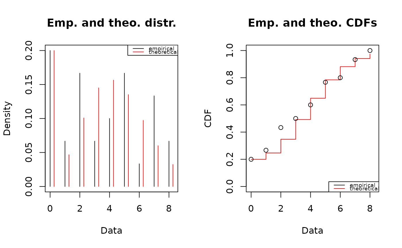
# (17) fit a non classical discrete distribution (the zero inflated Poisson distribution)
#
# \donttest{
require("gamlss.dist")
#> Loading required package: gamlss.dist
# depending of the random sample, the fit may fail
# it is why the seed was redefined here
# for you to get a sample on which it works
set.seed(1234)
x <- rZIP(n = 30, mu = 5, sigma = 0.2)
plotdist(x, discrete = TRUE)
# }
# (17) fit a non classical discrete distribution (the zero inflated Poisson distribution)
#
# \donttest{
require("gamlss.dist")
#> Loading required package: gamlss.dist
# depending of the random sample, the fit may fail
# it is why the seed was redefined here
# for you to get a sample on which it works
set.seed(1234)
x <- rZIP(n = 30, mu = 5, sigma = 0.2)
plotdist(x, discrete = TRUE)
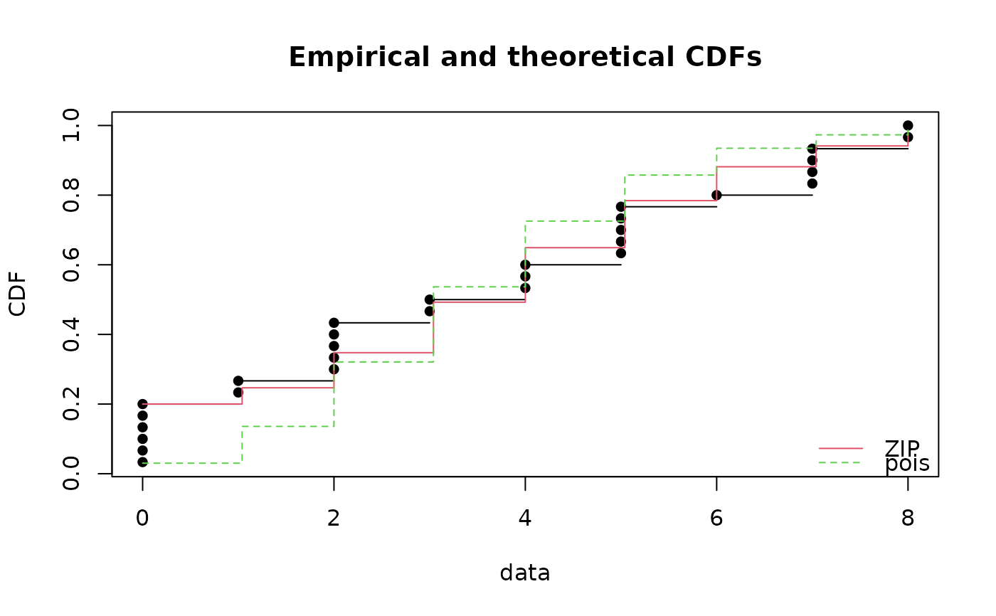
 fitzip <- fitdist(x, "ZIP", start = list(mu = 4, sigma = 0.15), discrete = TRUE,
optim.method = "L-BFGS-B", lower = c(0, 0), upper = c(Inf, 1))
#> Warning: The dZIP function should return a zero-length vector when input has length zero
#> Warning: The pZIP function should return a zero-length vector when input has length zero
summary(fitzip)
#> Fitting of the distribution ' ZIP ' by maximum likelihood
#> Parameters :
#> estimate Std. Error
#> mu 4.3166098 0.43412153
#> sigma 0.1891794 0.07416889
#> Loglikelihood: -67.13886 AIC: 138.2777 BIC: 141.0801
#> Correlation matrix:
#> mu sigma
#> mu 1.00000000 0.06418931
#> sigma 0.06418931 1.00000000
#>
plot(fitzip)
fitzip <- fitdist(x, "ZIP", start = list(mu = 4, sigma = 0.15), discrete = TRUE,
optim.method = "L-BFGS-B", lower = c(0, 0), upper = c(Inf, 1))
#> Warning: The dZIP function should return a zero-length vector when input has length zero
#> Warning: The pZIP function should return a zero-length vector when input has length zero
summary(fitzip)
#> Fitting of the distribution ' ZIP ' by maximum likelihood
#> Parameters :
#> estimate Std. Error
#> mu 4.3166098 0.43412153
#> sigma 0.1891794 0.07416889
#> Loglikelihood: -67.13886 AIC: 138.2777 BIC: 141.0801
#> Correlation matrix:
#> mu sigma
#> mu 1.00000000 0.06418931
#> sigma 0.06418931 1.00000000
#>
plot(fitzip)
 fitp <- fitdist(x, "pois")
cdfcomp(list(fitzip, fitp))
fitp <- fitdist(x, "pois")
cdfcomp(list(fitzip, fitp))
 gofstat(list(fitzip, fitp))
#> Chi-squared statistic: 3.579708 35.91516
#> Degree of freedom of the Chi-squared distribution: 3 4
#> Chi-squared p-value: 0.3105704 3.012341e-07
#> the p-value may be wrong with some theoretical counts < 5
#> Chi-squared table:
#> obscounts theo 1-mle-ZIP theo 2-mle-pois
#> <= 0 6 5.999996 0.9059215
#> <= 2 7 4.425507 8.7194943
#> <= 4 5 9.047522 12.1379326
#> <= 5 5 4.054142 3.9650580
#> <= 7 5 4.715294 3.4694258
#> > 7 2 1.757539 0.8021677
#>
#> Goodness-of-fit criteria
#> 1-mle-ZIP 2-mle-pois
#> Akaike's Information Criterion 138.2777 153.7397
#> Bayesian Information Criterion 141.0801 155.1409
# }
# (18) examples with distributions in actuar (predefined starting values)
#
# \donttest{
require("actuar")
x <- c(2.3,0.1,2.7,2.2,0.4,2.6,0.2,1.,7.3,3.2,0.8,1.2,33.7,14.,
21.4,7.7,1.,1.9,0.7,12.6,3.2,7.3,4.9,4000.,2.5,6.7,3.,63.,
6.,1.6,10.1,1.2,1.5,1.2,30.,3.2,3.5,1.2,0.2,1.9,0.7,17.,
2.8,4.8,1.3,3.7,0.2,1.8,2.6,5.9,2.6,6.3,1.4,0.8)
#log logistic
ft_llogis <- fitdist(x,'llogis')
x <- c(0.3837053, 0.8576858, 0.3552237, 0.6226119, 0.4783756, 0.3139799, 0.4051403,
0.4537631, 0.4711057, 0.5647414, 0.6479617, 0.7134207, 0.5259464, 0.5949068,
0.3509200, 0.3783077, 0.5226465, 1.0241043, 0.4384580, 1.3341520)
#inverse weibull
ft_iw <- fitdist(x,'invweibull')
# }
gofstat(list(fitzip, fitp))
#> Chi-squared statistic: 3.579708 35.91516
#> Degree of freedom of the Chi-squared distribution: 3 4
#> Chi-squared p-value: 0.3105704 3.012341e-07
#> the p-value may be wrong with some theoretical counts < 5
#> Chi-squared table:
#> obscounts theo 1-mle-ZIP theo 2-mle-pois
#> <= 0 6 5.999996 0.9059215
#> <= 2 7 4.425507 8.7194943
#> <= 4 5 9.047522 12.1379326
#> <= 5 5 4.054142 3.9650580
#> <= 7 5 4.715294 3.4694258
#> > 7 2 1.757539 0.8021677
#>
#> Goodness-of-fit criteria
#> 1-mle-ZIP 2-mle-pois
#> Akaike's Information Criterion 138.2777 153.7397
#> Bayesian Information Criterion 141.0801 155.1409
# }
# (18) examples with distributions in actuar (predefined starting values)
#
# \donttest{
require("actuar")
x <- c(2.3,0.1,2.7,2.2,0.4,2.6,0.2,1.,7.3,3.2,0.8,1.2,33.7,14.,
21.4,7.7,1.,1.9,0.7,12.6,3.2,7.3,4.9,4000.,2.5,6.7,3.,63.,
6.,1.6,10.1,1.2,1.5,1.2,30.,3.2,3.5,1.2,0.2,1.9,0.7,17.,
2.8,4.8,1.3,3.7,0.2,1.8,2.6,5.9,2.6,6.3,1.4,0.8)
#log logistic
ft_llogis <- fitdist(x,'llogis')
x <- c(0.3837053, 0.8576858, 0.3552237, 0.6226119, 0.4783756, 0.3139799, 0.4051403,
0.4537631, 0.4711057, 0.5647414, 0.6479617, 0.7134207, 0.5259464, 0.5949068,
0.3509200, 0.3783077, 0.5226465, 1.0241043, 0.4384580, 1.3341520)
#inverse weibull
ft_iw <- fitdist(x,'invweibull')
# }