Overview of the fitdistrplus package

Marie Laure Delignette Muller, Christophe Dutang

2024-10-26

Based on the article fitdistrplus: an R Package for Fitting Distributions (Marie Laure Delignette-Muller and Christophe Dutang, 2015, Journal of Statistical Software, DOI 10.18637/jss.v064.i04)

Keywords: probability distribution fitting, bootstrap, censored data, maximum likelihood, moment matching, quantile matching, maximum goodness-of-fit, distributions, R

1. Introduction

Fitting distributions to data is a very common task in statistics and consists in choosing a probability distribution modelling the random variable, as well as finding parameter estimates for that distribution. This requires judgment and expertise and generally needs an iterative process of distribution choice, parameter estimation, and quality of fit assessment. In the R (R Development Core Team 2013) package MASS (Venables and Ripley 2010), maximum likelihood estimation is available via the fitdistr function; other steps of the fitting process can be done using other R functions (Ricci 2005). In this paper, we present the R package fitdistrplus (Delignette-Muller et al. 2014) implementing several methods for fitting univariate parametric distribution. A first objective in developing this package was to provide R users a set of functions dedicated to help this overall process.

The fitdistr function estimates distribution parameters by maximizing the likelihood function using the optim function. No distinction between parameters with different roles (e.g., main parameter and nuisance parameter) is made, as this paper focuses on parameter estimation from a general point-of-view. In some cases, other estimation methods could be prefered, such as maximum goodness-of-fit estimation (also called minimum distance estimation), as proposed in the R package actuar with three different goodness-of-fit distances (Dutang, Goulet, and Pigeon 2008). While developping the fitdistrplus package, a second objective was to consider various estimation methods in addition to maximum likelihood estimation (MLE). Functions were developped to enable moment matching estimation (MME), quantile matching estimation (QME), and maximum goodness-of-fit estimation (MGE) using eight different distances. Moreover, the fitdistrplus package offers the possibility to specify a user-supplied function for optimization, useful in cases where classical optimization techniques, not included in optim, are more adequate.

In applied statistics, it is frequent to have to fit distributions to censored data Commeau et al. (2012). The MASS fitdistr function does not enable maximum likelihood estimation with this type of data. Some packages can be used to work with censored data, especially survival data Jordan (2005), but those packages generally focus on specific models, enabling the fit of a restricted set of distributions. A third objective is thus to provide R users a function to estimate univariate distribution parameters from right-, left- and interval-censored data.

Few packages on CRAN provide estimation procedures for any user-supplied parametric distribution and support different types of data. The distrMod package (Kohl and Ruckdeschel 2010) provides an object-oriented (S4) implementation of probability models and includes distribution fitting procedures for a given minimization criterion. This criterion is a user-supplied function which is sufficiently flexible to handle censored data, yet not in a trivial way, see Example M4 of the distrMod vignette. The fitting functions MLEstimator and MDEstimator return an S4 class for which a coercion method to class mle is provided so that the respective functionalities (e.g., confint and logLik) from package stats4 are available, too. In fitdistrplus, we chose to use the standard S3 class system for its understanding by most R users. When designing the fitdistrplus package, we did not forget to implement generic functions also available for S3 classes. Finally, various other packages provide functions to estimate the mode, the moments or the L-moments of a distribution, see the reference manuals of modeest, lmomco and Lmoments packages.

The package is available from the Comprehensive R Archive Network at . The paper is organized as follows: Section 2 presents tools for fitting continuous distributions to classic non-censored data. Section 3 deals with other estimation methods and other types of data, before Section 4 concludes.

2. Fitting distributions to continuous non-censored data

2.1. Choice of candidate distributions

For illustrating the use of various functions of the fitdistrplus package with continuous non-censored data, we will first use a data set named groundbeef which is included in our package. This data set contains pointwise values of serving sizes in grams, collected in a French survey, for ground beef patties consumed by children under 5 years old. It was used in a quantitative risk assessment published by Delignette-Muller and Cornu (2008).

require("fitdistrplus")

## Loading required package: fitdistrplus

## Loading required package: MASS

## Loading required package: survival

data("groundbeef")
str(groundbeef)

## 'data.frame':    254 obs. of  1 variable:
##  $ serving: num  30 10 20 24 20 24 40 20 50 30 ...

Before fitting one or more distributions to a data set, it is generally necessary to choose good candidates among a predefined set of distributions. This choice may be guided by the knowledge of stochastic processes governing the modeled variable, or, in the absence of knowledge regarding the underlying process, by the observation of its empirical distribution. To help the user in this choice, we developed functions to plot and characterize the empirical distribution.

First of all, it is common to start with plots of the empirical distribution function and the histogram (or density plot), which can be obtained with the plotdist function of the fitdistrplus package. This function provides two plots (see Figure @ref(fig:figgroundbeef)): the left-hand plot is by default the histogram on a density scale (or density plot of both, according to values of arguments histo and demp) and the right-hand plot the empirical cumulative distribution function (CDF).

plotdist(groundbeef$serving, histo = TRUE, demp = TRUE)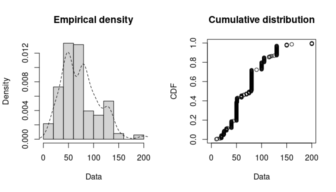

Histogram and CDF plots of an empirical distribution for a continuous variable (serving size from the groundbeef data set) as provided by the plotdist function.

In addition to empirical plots, descriptive statistics may help to choose candidates to describe a distribution among a set of parametric distributions. Especially the skewness and kurtosis, linked to the third and fourth moments, are useful for this purpose. A non-zero skewness reveals a lack of symmetry of the empirical distribution, while the kurtosis value quantifies the weight of tails in comparison to the normal distribution for which the kurtosis equals 3. The skewness and kurtosis and their corresponding unbiased estimator (Casella and Berger 2002) from a sample $(X_i)_i \stackrel{\text{i.i.d.}}{\sim} X$ with observations $(x_i)_i$ are given by:

$$\begin{equation} sk(X) = \frac{E[(X-E(X))^3]}{Var(X)^{\frac{3}{2}}}~,~\widehat{sk}=\frac{\sqrt{n(n-1)}}{n-2}\times\frac{m_{3}}{m_{2}^{\frac{3}{2}}},(\#eq:eq1) \end{equation}$$

$$\begin{equation} kr(X) = \frac{E[(X-E(X))^4]}{Var(X)^{2}}~,~\widehat{kr}=\frac{n-1}{(n-2)(n-3)}((n+1) \times \frac{m_{4}}{m_{2}^{2}}-3(n-1)) + 3,(\#eq:eq2) \end{equation}$$

where $m_{2}$, $m_{3}$, $m_{4}$ denote empirical moments defined by $m_{k}=\frac{1}{n}\sum_{i=1}^n(x_{i}-\overline{x})^{k}$, with $x_{i}$ the $n$ observations of variable $x$ and $\overline{x}$ their mean value.

The descdist function provides classical descriptive statistics (minimum, maximum, median, mean, standard deviation), skewness and kurtosis. By default, unbiased estimations of the three last statistics are provided. Nevertheless, the argument method can be changed from "unbiased" (default) to "sample" to obtain them without correction for bias. A skewness-kurtosis plot such as the one proposed by Cullen and Frey (1999) is provided by the descdist function for the empirical distribution (see Figure @ref(fig:descgroundbeefplot) for the groundbeef data set). On this plot, values for common distributions are displayed in order to help the choice of distributions to fit to data. For some distributions (normal, uniform, logistic, exponential), there is only one possible value for the skewness and the kurtosis. Thus, the distribution is represented by a single point on the plot. For other distributions, areas of possible values are represented, consisting in lines (as for gamma and lognormal distributions), or larger areas (as for beta distribution).

Skewness and kurtosis are known not to be robust. In order to take into account the uncertainty of the estimated values of kurtosis and skewness from data, a nonparametric bootstrap procedure (Efron and Tibshirani 1994) can be performed by using the argument boot. Values of skewness and kurtosis are computed on bootstrap samples (constructed by random sampling with replacement from the original data set) and reported on the skewness-kurtosis plot. Nevertheless, the user needs to know that skewness and kurtosis, like all higher moments, have a very high variance. This is a problem which cannot be completely solved by the use of bootstrap. The skewness-kurtosis plot should then be regarded as indicative only. The properties of the random variable should be considered, notably its expected value and its range, as a complement to the use of the plotdist and descdist functions. Below is a call to the descdist function to describe the distribution of the serving size from the groundbeef data set and to draw the corresponding skewness-kurtosis plot (see Figure @ref(fig:descgroundbeefplot)). Looking at the results on this example with a positive skewness and a kurtosis not far from 3, the fit of three common right-skewed distributions could be considered, Weibull, gamma and lognormal distributions.

descdist(groundbeef$serving, boot = 1000)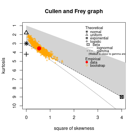

Skewness-kurtosis plot for a continuous variable (serving size from the groundbeef data set) as provided by the descdist function.

## summary statistics
## ------
## min:  10   max:  200 
## median:  79 
## mean:  73.65 
## estimated sd:  35.88 
## estimated skewness:  0.7353 
## estimated kurtosis:  3.551

2.2. Fit of distributions by maximum likelihood estimation

Once selected, one or more parametric distributions $f(.\vert \theta)$ (with parameter $\theta\in\mathbb{R}^d$) may be fitted to the data set, one at a time, using the fitdist function. Under the i.i.d. sample assumption, distribution parameters $\theta$ are by default estimated by maximizing the likelihood function defined as:

$$\begin{equation} L(\theta)=\prod_{i=1}^n f(x_{i}\vert \theta)(\#eq:eq3) \end{equation}$$

with $x_{i}$ the $n$ observations of variable $X$ and $f(.\vert \theta)$ the density function of the parametric distribution. The other proposed estimation methods are described in Section 3.1..

The fitdist function returns an S3 object of class fitdist for which print, summary and plot functions are provided. The fit of a distribution using fitdist assumes that the corresponding d, p, q functions (standing respectively for the density, the distribution and the quantile functions) are defined. Classical distributions are already defined in that way in the stats package, e.g., dnorm, pnorm and qnorm for the normal distribution (see ?Distributions). Others may be found in various packages (see the CRAN task view: Probability Distributions at ). Distributions not found in any package must be implemented by the user as d, p, q functions. In the call to fitdist, a distribution has to be specified via the argument dist either by the character string corresponding to its common root name used in the names of d, p, q functions (e.g., "norm" for the normal distribution) or by the density function itself, from which the root name is extracted (e.g., dnorm for the normal distribution). Numerical results returned by the fitdist function are (1) the parameter estimates, (2) the estimated standard errors (computed from the estimate of the Hessian matrix at the maximum likelihood solution), (3) the loglikelihood, (4) Akaike and Bayesian information criteria (the so-called AIC and BIC), and (5) the correlation matrix between parameter estimates. Below is a call to the fitdist function to fit a Weibull distribution to the serving size from the groundbeef data set.

fw <- fitdist(groundbeef$serving, "weibull")
summary(fw)

## Fitting of the distribution ' weibull ' by maximum likelihood 
## Parameters : 
##       estimate Std. Error
## shape    2.186      1.667
## scale   83.348     40.272
## Loglikelihood:  -1255   AIC:  2514   BIC:  2522 
## Correlation matrix:
##        shape  scale
## shape 1.0000 0.3218
## scale 0.3218 1.0000

The plot of an object of class fitdist provides four classical goodness-of-fit plots (Cullen and Frey 1999) presented on Figure @ref(fig:groundbeefcomp):

• a density plot representing the density function of the fitted distribution along with the histogram of the empirical distribution,
• a CDF plot of both the empirical distribution and the fitted distribution,
• a Q-Q plot representing the empirical quantiles (y-axis) against the theoretical quantiles (x-axis),
• a P-P plot representing the empirical distribution function evaluated at each data point (y-axis) against the fitted distribution function (x-axis).

For CDF, Q-Q and P-P plots, the probability plotting position is defined by default using Hazen’s rule, with probability points of the empirical distribution calculated as (1:n - 0.5)/n, as recommended by Blom (1959). This plotting position can be easily changed (see the reference manual for details (Delignette-Muller et al. 2014)).

Unlike the generic plot function, the denscomp, cdfcomp, qqcomp and ppcomp functions enable to draw separately each of these four plots, in order to compare the empirical distribution and multiple parametric distributions fitted on a same data set. These functions must be called with a first argument corresponding to a list of objects of class fitdist, and optionally further arguments to customize the plot (see the reference manual for lists of arguments that may be specific to each plot (Delignette-Muller et al. 2014)). In the following example, we compare the fit of a Weibull, a lognormal and a gamma distributions to the groundbeef data set (Figure @ref(fig:groundbeefcomp)).

par(mfrow = c(2, 2), mar = c(4, 4, 2, 1))
fg <- fitdist(groundbeef$serving, "gamma")
fln <- fitdist(groundbeef$serving, "lnorm")
plot.legend <- c("Weibull", "lognormal", "gamma")
denscomp(list(fw, fln, fg), legendtext = plot.legend)
qqcomp(list(fw, fln, fg), legendtext = plot.legend)
cdfcomp(list(fw, fln, fg), legendtext = plot.legend)
ppcomp(list(fw, fln, fg), legendtext = plot.legend)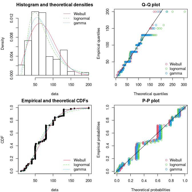

Four Goodness-of-fit plots for various distributions fitted to continuous data (Weibull, gamma and lognormal distributions fitted to serving sizes from the groundbeef data set) as provided by functions denscomp, qqcomp, cdfcomp and ppcomp.

The density plot and the CDF plot may be considered as the basic classical goodness-of-fit plots. The two other plots are complementary and can be very informative in some cases. The Q-Q plot emphasizes the lack-of-fit at the distribution tails while the P-P plot emphasizes the lack-of-fit at the distribution center. In the present example (in Figure @ref(fig:groundbeefcomp)), none of the three fitted distributions correctly describes the center of the distribution, but the Weibull and gamma distributions could be prefered for their better description of the right tail of the empirical distribution, especially if this tail is important in the use of the fitted distribution, as it is in the context of food risk assessment.

The data set named endosulfan will now be used to illustrate other features of the fitdistrplus package. This data set contains acute toxicity values for the organochlorine pesticide endosulfan (geometric mean of LC50 ou EC50 values in $\mu g.L^{-1}$), tested on Australian and non-Australian laboratory-species (Hose and Van den Brink 2004). In ecotoxicology, a lognormal or a loglogistic distribution is often fitted to such a data set in order to characterize the species sensitivity distribution (SSD) for a pollutant. A low percentile of the fitted distribution, generally the 5% percentile, is then calculated and named the hazardous concentration 5% (HC5). It is interpreted as the value of the pollutant concentration protecting 95% of the species (Posthuma, Suter, and Traas 2010). But the fit of a lognormal or a loglogistic distribution to the whole endosulfan data set is rather bad (Figure @ref(fig:fitendo)), especially due to a minority of very high values. The two-parameter Pareto distribution and the three-parameter Burr distribution (which is an extension of both the loglogistic and the Pareto distributions) have been fitted. Pareto and Burr distributions are provided in the package actuar. Until here, we did not have to define starting values (in the optimization process) as reasonable starting values are implicity defined within the fitdist function for most of the distributions defined in R (see ?fitdist for details). For other distributions like the Pareto and the Burr distribution, initial values for the distribution parameters have to be supplied in the argument start, as a named list with initial values for each parameter (as they appear in the d, p, q functions). Having defined reasonable starting values¹ various distributions can be fitted and graphically compared. On this example, the function cdfcomp can be used to report CDF values in a logscale so as to emphasize discrepancies on the tail of interest while defining an HC5 value (Figure @ref(fig:fitendo)).

require("actuar")

## Loading required package: actuar

## 
## Attaching package: 'actuar'

## The following objects are masked from 'package:stats':
## 
##     sd, var

## The following object is masked from 'package:grDevices':
## 
##     cm

data("endosulfan")
ATV <- endosulfan$ATV
fendo.ln <- fitdist(ATV, "lnorm")
fendo.ll <- fitdist(ATV, "llogis", start = list(shape = 1, scale = 500))
fendo.P <- fitdist(ATV, "pareto", start = list(shape = 1, scale = 500))
fendo.B <- fitdist(ATV, "burr", start = list(shape1 = 0.3, shape2 = 1, rate = 1))
cdfcomp(list(fendo.ln, fendo.ll, fendo.P, fendo.B), xlogscale = TRUE, 
        ylogscale = TRUE, legendtext = c("lognormal", "loglogistic", "Pareto", "Burr"))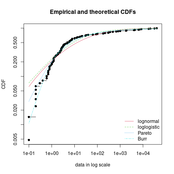

CDF plot to compare the fit of four distributions to acute toxicity values of various organisms for the organochlorine pesticide endosulfan (endosulfan data set) as provided by the cdfcomp function, with CDF values in a logscale to emphasize discrepancies on the left tail.

None of the fitted distribution correctly describes the right tail observed in the data set, but as shown in Figure @ref(fig:fitendo), the left-tail seems to be better described by the Burr distribution. Its use could then be considered to estimate the HC5 value as the 5% quantile of the distribution. This can be easily done using the quantile generic function defined for an object of class fitdist. Below is this calculation together with the calculation of the empirical quantile for comparison.

quantile(fendo.B, probs = 0.05)

## Estimated quantiles for each specified probability (non-censored data)
##          p=0.05
## estimate 0.2939

quantile(ATV, probs = 0.05)

##  5% 
## 0.2

In addition to the ecotoxicology context, the quantile generic function is also attractive in the actuarial-financial context. In fact, the value-at-risk $VAR_\alpha$ is defined as the $1-\alpha$-quantile of the loss distribution and can be computed with quantile on a fitdist object.

The computation of different goodness-of-fit statistics is proposed in the fitdistrplus package in order to further compare fitted distributions. The purpose of goodness-of-fit statistics aims to measure the distance between the fitted parametric distribution and the empirical distribution: e.g., the distance between the fitted cumulative distribution function $F$ and the empirical distribution function $F_{n}$. When fitting continuous distributions, three goodness-of-fit statistics are classicaly considered: Cramer-von Mises, Kolmogorov-Smirnov and Anderson-Darling statistics (D’Agostino and Stephens 1986). Naming $x_{i}$ the $n$ observations of a continuous variable $X$ arranged in an ascending order, Table @ref(tab:tabKSCvMAD) gives the definition and the empirical estimate of the three considered goodness-of-fit statistics. They can be computed using the function gofstat as defined by Stephens (D’Agostino and Stephens 1986).

gofstat(list(fendo.ln, fendo.ll, fendo.P, fendo.B), 
        fitnames = c("lnorm", "llogis", "Pareto", "Burr"))

## Goodness-of-fit statistics
##                               lnorm llogis  Pareto    Burr
## Kolmogorov-Smirnov statistic 0.1672 0.1196 0.08488 0.06155
## Cramer-von Mises statistic   0.6374 0.3827 0.13926 0.06803
## Anderson-Darling statistic   3.4721 2.8316 0.89206 0.52393
## 
## Goodness-of-fit criteria
##                                lnorm llogis Pareto Burr
## Akaike's Information Criterion  1069   1069   1048 1046
## Bayesian Information Criterion  1074   1075   1053 1054

(#tab:tabKSCvMAD) Goodness-of-fit statistics as defined by Stephens (D’Agostino and Stephens 1986).

Statistic	General formula	Computational formula
Kolmogorov-Smirnov (KS)	$\sup|F_{n}(x) - F(x)|$	$\max(D^{+},D^{-})$ with $D^{+}=\max\limits_{i=1,\dots,n}\left(\frac{i}{n} - F_i\right)$ and $D^{-}=\max\limits_{i=1,\dots,n}\left(F_{i}-\frac{i-1}{n}\right)$
Cramer-von Mises (CvM)	$n \int_{-\infty}^{\infty}(F_{n}(x) - F(x))^2 dx$	$\frac{1}{12n} + \sum\limits_{i=1}^n \left(F_i-\frac{2i-1}{2n} \right)^{2}$
Anderson-Darling (AD)	$n \int_{-\infty}^{\infty}\frac{(F_{n}(x) - F(x))^2}{F(x) (1 - F(x))} dx$	$-n -\frac{1}{n}\sum\limits_{i=1}^n (2i-1)\log(F_i(1-F_{n+1-i}))$

where $F_i\stackrel{\triangle}{=} F(x_i)$

As giving more weight to distribution tails, the Anderson-Darling statistic is of special interest when it matters to equally emphasize the tails as well as the main body of a distribution. This is often the case in risk assessment Vose (2010). For this reason, this statistics is often used to select the best distribution among those fitted. Nevertheless, this statistics should be used cautiously when comparing fits of various distributions. Keeping in mind that the weighting of each CDF quadratic difference depends on the parametric distribution in its definition (see Table @ref(tab:tabKSCvMAD)), Anderson-Darling statistics computed for several distributions fitted on a same data set are theoretically difficult to compare. Moreover, such a statistic, as Cramer-von Mises and Kolmogorov-Smirnov ones, does not take into account the complexity of the model (i.e., parameter number). It is not a problem when compared distributions are characterized by the same number of parameters, but it could systematically promote the selection of the more complex distributions in the other case. Looking at classical penalized criteria based on the loglikehood (AIC, BIC) seems thus also interesting, especially to discourage overfitting.

In the previous example, all the goodness-of-fit statistics based on the CDF distance are in favor of the Burr distribution, the only one characterized by three parameters, while AIC and BIC values respectively give the preference to the Burr distribution or the Pareto distribution. The choice between these two distributions seems thus less obvious and could be discussed. Even if specifically recommended for discrete distributions, the Chi-squared statistic may also be used for continuous distributions (see Section 3.3. and the reference manual for examples (Delignette-Muller et al. 2014)).

2.3. Uncertainty in parameter estimates

The uncertainty in the parameters of the fitted distribution can be estimated by parametric or nonparametric bootstraps using the boodist function for non-censored data (Efron and Tibshirani 1994). This function returns the bootstrapped values of parameters in an S3 class object which can be plotted to visualize the bootstrap region. The medians and the 95% confidence intervals of parameters (2.5 and 97.5 percentiles) are printed in the summary. When inferior to the whole number of iterations (due to lack of convergence of the optimization algorithm for some bootstrapped data sets), the number of iterations for which the estimation converges is also printed in the summary.

The plot of an object of class bootdist consists in a scatterplot or a matrix of scatterplots of the bootstrapped values of parameters providing a representation of the joint uncertainty distribution of the fitted parameters. Below is an example of the use of the bootdist function with the previous fit of the Burr distribution to the endosulfan data set (Figure @ref(fig:bootstrap)).

bendo.B <- bootdist(fendo.B, niter = 1001)
summary(bendo.B)

## Parametric bootstrap medians and 95% percentile CI 
##        Median    2.5%  97.5%
## shape1 0.1983 0.09283 0.3606
## shape2 1.5863 1.05306 3.0629
## rate   1.4907 0.70828 2.7775

plot(bendo.B)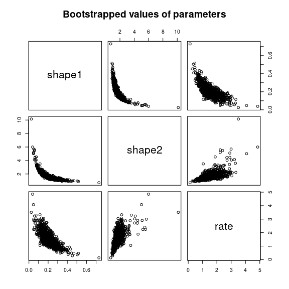

Bootstrappped values of parameters for a fit of the Burr distribution characterized by three parameters (example on the endosulfan data set) as provided by the plot of an object of class bootdist.

Bootstrap samples of parameter estimates are useful especially to calculate confidence intervals on each parameter of the fitted distribution from the marginal distribution of the bootstraped values. It is also interesting to look at the joint distribution of the bootstraped values in a scatterplot (or a matrix of scatterplots if the number of parameters exceeds two) in order to understand the potential structural correlation between parameters (see Figure @ref(fig:bootstrap)).

The use of the whole bootstrap sample is also of interest in the risk assessment field. Its use enables the characterization of uncertainty in distribution parameters. It can be directly used within a second-order Monte Carlo simulation framework, especially within the package mc2d (Pouillot, Delignette-Muller, and Denis 2011). One could refer to Pouillot and Delignette-Muller (2010) for an introduction to the use of mc2d and fitdistrplus packages in the context of quantitative risk assessment.

The bootstrap method can also be used to calculate confidence intervals on quantiles of the fitted distribution. For this purpose, a generic quantile function is provided for class bootdist. By default, 95% percentiles bootstrap confidence intervals of quantiles are provided. Going back to the previous example from ecotoxicolgy, this function can be used to estimate the uncertainty associated to the HC5 estimation, for example from the previously fitted Burr distribution to the endosulfan data set.

quantile(bendo.B, probs = 0.05)

## (original) estimated quantiles for each specified probability (non-censored data)
##          p=0.05
## estimate 0.2939
## Median of bootstrap estimates
##          p=0.05
## estimate 0.2994
## 
## two-sided 95 % CI of each quantile
##        p=0.05
## 2.5 %  0.1792
## 97.5 % 0.4999

3. Advanced topics

3.1. Alternative methods for parameter estimation

This subsection focuses on alternative estimation methods. One of the alternative for continuous distributions is the maximum goodness-of-fit estimation method also called minimum distance estimation method Dutang, Goulet, and Pigeon (2008). In this package this method is proposed with eight different distances: the three classical distances defined in Table @ref(tab:tabKSCvMAD), or one of the variants of the Anderson-Darling distance proposed by Luceno (2006) and defined in Table @ref(tab:modifiedAD). The right-tail AD gives more weight to the right-tail, the left-tail AD gives more weight only to the left tail. Either of the tails, or both of them, can receive even larger weights by using second order Anderson-Darling Statistics.

(#tab:modifiedAD) Modified Anderson-Darling statistics as defined by Luceno (2006).

Statistic	General formula	Computational formula
Right-tail AD (ADR)	$\int_{-\infty}^{\infty}\frac{(F_{n}(x) - F(x))^2 }{1 - F(x)} dx$	$\frac{n}{2} -2\sum\limits_{i=1}^nF_i -\frac{1}{n}\sum\limits_{i=1}^n(2i-1)ln(\overline F_{n+1-i})$
Left-tail AD (ADL)	$\int_{-\infty}^{\infty}\frac{(F_{n}(x) - F(x))^2 }{(F(x))} dx$	$-\frac{3n}{2} +2\sum\limits_{i=1}^nF_i -\frac{1}{n}\sum\limits_{i=1}^n(2i-1)ln(F_i)$
Right-tail AD 2nd order (AD2R)	$ad2r=\int_{-\infty}^{\infty}\frac{(F_{n}(x) - F(x))^2 }{(1 - F(x))^{2}} dx$	$ad2r=2\sum\limits_{i=1}^nln(\overline F_i) +\frac{1}{n}\sum\limits_{i=1}^n \frac{2i-1}{\overline F_{n+1-i}}$
Left-tail AD 2nd order (AD2L)	$ad2l=\int_{-\infty}^{\infty}\frac{(F_{n}(x) - F(x))^2 }{(F(x))^{2}} dx$	$ad2l=2\sum\limits_{i=1}^nln(F_i) +\frac{1}{n}\sum\limits_{i=1}^n\frac{2i-1}{F_i}$
AD 2nd order (AD2)	$ad2r+ad2l$	$ad2r+ad2l$

where $F_i\stackrel{\triangle}{=} F(x_{i})$ and $\overline F_i\stackrel{\triangle}{=}1-F(x_{i})$

To fit a distribution by maximum goodness-of-fit estimation, one needs to fix the argument method to mge in the call to fitdist and to specify the argument gof coding for the chosen goodness-of-fit distance. This function is intended to be used only with continuous non-censored data.

Maximum goodness-of-fit estimation may be useful to give more weight to data at one tail of the distribution. In the previous example from ecotoxicology, we used a non classical distribution (the Burr distribution) to correctly fit the empirical distribution especially on its left tail. In order to correctly estimate the 5$\%$ percentile, we could also consider the fit of the classical lognormal distribution, but minimizing a goodness-of-fit distance giving more weight to the left tail of the empirical distribution. In what follows, the left tail Anderson-Darling distances of first or second order are used to fit a lognormal to endosulfan data set (see Figure @ref(fig:plotfitMGE)).

fendo.ln.ADL <- fitdist(ATV, "lnorm", method = "mge", gof = "ADL")
fendo.ln.AD2L <- fitdist(ATV, "lnorm", method = "mge", gof = "AD2L")
cdfcomp(list(fendo.ln, fendo.ln.ADL, fendo.ln.AD2L), 
  xlogscale = TRUE, ylogscale = TRUE, 
  main = "Fitting a lognormal distribution",
  xlegend = "bottomright", 
  legendtext = c("MLE", "Left-tail AD", "Left-tail AD 2nd order"))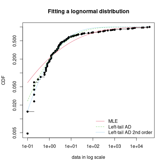

Comparison of a lognormal distribution fitted by MLE and by MGE using two different goodness-of-fit distances: left-tail Anderson-Darling and left-tail Anderson Darling of second order (example with the endosulfan data set) as provided by the cdfcomp function, with CDF values in a logscale to emphasize discrepancies on the left tail.

Comparing the 5% percentiles (HC5) calculated using these three fits to the one calculated from the MLE fit of the Burr distribution, we can observe, on this example, that fitting the lognormal distribution by maximizing left tail Anderson-Darling distances of first or second order enables to approach the value obtained by fitting the Burr distribution by MLE.

(HC5.estimates <- c(
  empirical = as.numeric(quantile(ATV, probs = 0.05)), 
  Burr = as.numeric(quantile(fendo.B, probs = 0.05)$quantiles), 
  lognormal_MLE = as.numeric(quantile(fendo.ln, probs = 0.05)$quantiles), 
  lognormal_AD2 = as.numeric(quantile(fendo.ln.ADL, probs = 0.05)$quantiles), 
  lognormal_AD2L = as.numeric(quantile(fendo.ln.AD2L, probs = 0.05)$quantiles)))

##      empirical           Burr  lognormal_MLE  lognormal_AD2 lognormal_AD2L 
##        0.20000        0.29393        0.07259        0.19591        0.25877

The moment matching estimation (MME) is another method commonly used to fit parametric distributions (Vose 2010). MME consists in finding the value of the parameter $\theta$ that equalizes the first theoretical raw moments of the parametric distribution to the corresponding empirical raw moments as in Equation @ref(eq:eq4):

$$\begin{equation} E(X^{k}|\theta)=\frac{1}{n}\sum_{i=1}^{n}x_{i}^{k},(\#eq:eq4) \end{equation}$$ for $k=1,\ldots,d$, with $d$ the number of parameters to estimate and $x_{i}$ the $n$ observations of variable $X$. For moments of order greater than or equal to 2, it may also be relevant to match centered moments. Therefore, we match the moments given in Equation @ref(eq:eq5):

$$\begin{equation} E(X\vert \theta) = \overline{x} ~,~E\left((X-E(X))^{k}|\theta\right)=m_k, \text{ for } k=2,\ldots,d,(\#eq:eq5) \end{equation}$$

where $m_k$ denotes the empirical centered moments. This method can be performed by setting the argument method to "mme" in the call to fitdist. The estimate is computed by a closed-form formula for the following distributions: normal, lognormal, exponential, Poisson, gamma, logistic, negative binomial, geometric, beta and uniform distributions. In this case, for distributions characterized by one parameter (geometric, Poisson and exponential), this parameter is simply estimated by matching theoretical and observed means, and for distributions characterized by two parameters, these parameters are estimated by matching theoretical and observed means and variances (Vose 2010). For other distributions, the equation of moments is solved numerically using the optim function by minimizing the sum of squared differences between observed and theoretical moments (see the fitdistrplus reference manual for technical details (Delignette-Muller et al. 2014)).

A classical data set from the Danish insurance industry published in McNeil (1997) will be used to illustrate this method. In fitdistrplus, the data set is stored in danishuni for the univariate version and contains the loss amounts collected at Copenhagen Reinsurance between 1980 and 1990. In actuarial science, it is standard to consider positive heavy-tailed distributions and have a special focus on the right-tail of the distributions. In this numerical experiment, we choose classic actuarial distributions for loss modelling: the lognormal distribution and the Pareto type II distribution (Klugman, Panjer, and Willmot 2009).

The lognormal distribution is fitted to danishuni data set by matching moments implemented as a closed-form formula. On the left-hand graph of Figure @ref(fig:danishmme), the fitted distribution functions obtained using the moment matching estimation (MME) and maximum likelihood estimation (MLE) methods are compared. The MME method provides a more cautious estimation of the insurance risk as the MME-fitted distribution function (resp. MLE-fitted) underestimates (overestimates) the empirical distribution function for large values of claim amounts.

data("danishuni")
str(danishuni)

## 'data.frame':    2167 obs. of  2 variables:
##  $ Date: Date, format: "1980-01-03" "1980-01-04" ...
##  $ Loss: num  1.68 2.09 1.73 1.78 4.61 ...

fdanish.ln.MLE <- fitdist(danishuni$Loss, "lnorm")
fdanish.ln.MME <- fitdist(danishuni$Loss, "lnorm", method = "mme", order = 1:2)
require("actuar")
fdanish.P.MLE <- fitdist(danishuni$Loss, "pareto", start = list(shape = 10, scale = 10), 
                         lower = 2+1e-6, upper = Inf)

## Warning in cov2cor(varcovar): diag(V) had non-positive or NA entries; the
## non-finite result may be dubious

## Warning in sqrt(diag(varcovar)): NaNs produced

memp <- function(x, order) mean(x^order)
fdanish.P.MME <- fitdist(danishuni$Loss, "pareto", method = "mme", order = 1:2, memp = "memp", 
                         start = list(shape = 10, scale = 10), lower = c(2+1e-6, 2+1e-6), 
                         upper = c(Inf, Inf))

## Warning in cov2cor(varcovar): diag(V) had non-positive or NA entries; the
## non-finite result may be dubious

par(mfrow = c(1, 2))
cdfcomp(list(fdanish.ln.MLE, fdanish.ln.MME), legend = c("lognormal MLE", "lognormal MME"),
        main = "Fitting a lognormal distribution", xlogscale = TRUE, datapch = 20)
cdfcomp(list(fdanish.P.MLE, fdanish.P.MME), legend = c("Pareto MLE", "Pareto MME"), 
        main = "Fitting a Pareto distribution", xlogscale = TRUE, datapch = 20)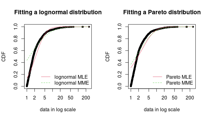

Comparison between MME and MLE when fitting a lognormal or a Pareto distribution to loss data from the danishuni data set.

In a second time, a Pareto distribution, which gives more weight to the right-tail of the distribution, is fitted. As the lognormal distribution, the Pareto has two parameters, which allows a fair comparison.

We use the implementation of the actuar package providing raw and centered moments for that distribution (in addition to d, p, q and r functions (Goulet 2012). Fitting a heavy-tailed distribution for which the first and the second moments do not exist for certain values of the shape parameter requires some cautiousness. This is carried out by providing, for the optimization process, a lower and an upper bound for each parameter. The code below calls the L-BFGS-B optimization method in optim, since this quasi-Newton allows box constraints ². We choose match moments defined in Equation @ref(eq:eq4), and so a function for computing the empirical raw moment (called memp in our example) is passed to fitdist. For two-parameter distributions (i.e., $d=2$), Equations @ref(eq:eq4) and @ref(eq:eq5) are equivalent.

gofstat(list(fdanish.ln.MLE, fdanish.P.MLE, fdanish.ln.MME, fdanish.P.MME), 
        fitnames = c("lnorm.mle", "Pareto.mle", "lnorm.mme", "Pareto.mme"))

## Goodness-of-fit statistics
##                              lnorm.mle Pareto.mle lnorm.mme Pareto.mme
## Kolmogorov-Smirnov statistic    0.1375     0.3124    0.4368       0.37
## Cramer-von Mises statistic     14.7911    37.7166   88.9503      55.43
## Anderson-Darling statistic     87.1933   208.3143  416.2567     281.58
## 
## Goodness-of-fit criteria
##                                lnorm.mle Pareto.mle lnorm.mme Pareto.mme
## Akaike's Information Criterion      8120       9250      9792       9409
## Bayesian Information Criterion      8131       9261      9803       9420

As shown on Figure @ref(fig:danishmme), MME and MLE fits are far less distant (when looking at the right-tail) for the Pareto distribution than for the lognormal distribution on this data set. Furthermore, for these two distributions, the MME method better fits the right-tail of the distribution from a visual point of view. This seems logical since empirical moments are influenced by large observed values. In the previous traces, we gave the values of goodness-of-fit statistics. Whatever the statistic considered, the MLE-fitted lognormal always provides the best fit to the observed data.

Maximum likelihood and moment matching estimations are certainly the most commonly used method for fitting distributions (Cullen and Frey 1999). Keeping in mind that these two methods may produce very different results, the user should be aware of its great sensitivity to outliers when choosing the moment matching estimation. This may be seen as an advantage in our example if the objective is to better describe the right tail of the distribution, but it may be seen as a drawback if the objective is different.

Fitting of a parametric distribution may also be done by matching theoretical quantiles of the parametric distributions (for specified probabilities) against the empirical quantiles (Tse 2009). The equality of theoretical and empirical quantiles is expressed by Equation @ref(eq:eq6) below, which is very similar to Equations @ref(eq:eq4) and @ref(eq:eq5):

$$\begin{equation} F^{-1}(p_{k}|\theta)=Q_{n,p_{k}}(\#eq:eq6) \end{equation}$$ for $k=1,\ldots,d$, with $d$ the number of parameters to estimate (dimension of $\theta$ if there is no fixed parameters) and $Q_{n,p_{k}}$ the empirical quantiles calculated from data for specified probabilities $p_{k}$.

Quantile matching estimation (QME) is performed by setting the argument method to "qme" in the call to fitdist and adding an argument probs defining the probabilities for which the quantile matching is performed (see Figure @ref(fig:danishqme)). The length of this vector must be equal to the number of parameters to estimate (as the vector of moment orders for MME). Empirical quantiles are computed using the quantile function of the stats package using type=7 by default (see ?quantile and Hyndman and Fan (1996)). But the type of quantile can be easily changed by using the qty argument in the call to the qme function.
The quantile matching is carried out numerically, by minimizing the sum of squared differences between observed and theoretical quantiles.

fdanish.ln.QME1 <- fitdist(danishuni$Loss, "lnorm", method = "qme", probs = c(1/3, 2/3))
fdanish.ln.QME2 <- fitdist(danishuni$Loss, "lnorm", method = "qme", probs = c(8/10, 9/10))
cdfcomp(list(fdanish.ln.MLE, fdanish.ln.QME1, fdanish.ln.QME2), 
        legend = c("MLE", "QME(1/3, 2/3)", "QME(8/10, 9/10)"), 
        main = "Fitting a lognormal distribution", xlogscale = TRUE, datapch = 20)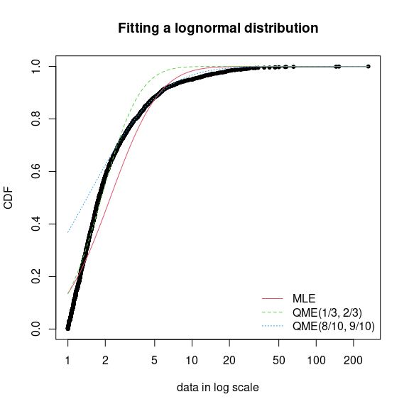

Comparison between QME and MLE when fitting a lognormal distribution to loss data from the danishuni data set.

Above is an example of fitting of a lognormal distribution to `danishuni} data set by matching probabilities $(p_1= 1/3, p_2=2/3)$ and $(p_1= 8/10, p_2=9/10)$. As expected, the second QME fit gives more weight to the right-tail of the distribution. Compared to the maximum likelihood estimation, the second QME fit best suits the right-tail of the distribution, whereas the first QME fit best models the body of the distribution. The quantile matching estimation is of particular interest when we need to focus around particular quantiles, e.g., $p=99.5\%$ in the Solvency II insurance context or $p=5\%$ for the HC5 estimation in the ecotoxicology context.

3.2. Customization of the optimization algorithm

Each time a numerical minimization is carried out in the fitdistrplus package, the optim function of the stats package is used by default with the Nelder-Mead method for distributions characterized by more than one parameter and the BFGS method for distributions characterized by only one parameter. Sometimes the default algorithm fails to converge. It is then interesting to change some options of the optim function or to use another optimization function than optim to minimize the objective function. The argument optim.method can be used in the call to fitdist or fitdistcens. It will internally be passed to mledist, mmedist, mgedist or qmedist, and to optim (see ?optim for details about the different algorithms available).

Even if no error is raised when computing the optimization, changing the algorithm is of particular interest to enforce bounds on some parameters. For instance, a volatility parameter $\sigma$ is strictly positive $\sigma>0$ and a probability parameter $p$ lies in $p\in [0,1]$. This is possible by using arguments lower and/or upper, for which their use automatically forces optim.method="L-BFGS-B".

Below are examples of fits of a gamma distribution $\mathcal{G}(\alpha, \lambda)$ to the groundbeef data set with various algorithms. Note that the conjugate gradient algorithm (CG) needs far more iterations to converge (around 2500 iterations) compared to other algorithms (converging in less than 100 iterations).

data("groundbeef")
fNM <- fitdist(groundbeef$serving, "gamma", optim.method = "Nelder-Mead")
fBFGS <- fitdist(groundbeef$serving, "gamma", optim.method = "BFGS") 
fSANN <- fitdist(groundbeef$serving, "gamma", optim.method = "SANN")
fCG <- try(fitdist(groundbeef$serving, "gamma", optim.method = "CG",
                   control = list(maxit = 10000)))
if(inherits(fCG, "try-error")) {fCG <- list(estimate = NA)}

It is also possible to use another function than optim to minimize the objective function by specifying by the argument custom.optim in the call to fitdist. It may be necessary to customize this optimization function to meet the following requirements. (1) custom.optim function must have the following arguments: fn for the function to be optimized and par for the initialized parameters. (2) custom.optim should carry out a MINIMIZATION and must return the following components: par for the estimate, convergence for the convergence code, value=fn(par) and hessian. Below is an example of code written to wrap the genoud function from the rgenoud package in order to respect our optimization ``template’’. The rgenoud package implements the genetic (stochastic) algorithm.

mygenoud <- function(fn, par, ...) 
{
   require("rgenoud")
   res <- genoud(fn, starting.values = par, ...)        
   standardres <- c(res, convergence = 0)
   return(standardres)
}

The customized optimization function can then be passed as the argument custom.optim in the call to fitdist or fitdistcens. The following code can for example be used to fit a gamma distribution to the groundbeef data set. Note that in this example various arguments are also passed from fitdist to genoud: nvars, Domains, boundary.enforcement, print.level and hessian. The code below compares all the parameter estimates ($\hat\alpha$, $\hat\lambda$) by the different algorithms: shape $\alpha$ and rate $\lambda$ parameters are relatively similar on this example, roughly 4.00 and 0.05, respectively.

fgenoud <- mledist(groundbeef$serving, "gamma", custom.optim = mygenoud, nvars = 2, 
                   max.generations = 10, Domains = cbind(c(0, 0), c(10, 10)), 
                   boundary.enforcement = 1, hessian = TRUE, print.level = 0, P9 = 10)

## Loading required package: rgenoud

## ##  rgenoud (Version 5.9-0.11, Build Date: 2024-10-03)
## ##  See http://sekhon.berkeley.edu/rgenoud for additional documentation.
## ##  Please cite software as:
## ##   Walter Mebane, Jr. and Jasjeet S. Sekhon. 2011.
## ##   ``Genetic Optimization Using Derivatives: The rgenoud package for R.''
## ##   Journal of Statistical Software, 42(11): 1-26. 
## ##

cbind(NM = fNM$estimate, BFGS = fBFGS$estimate, SANN = fSANN$estimate, CG = fCG$estimate, 
      fgenoud = fgenoud$estimate)

##            NM    BFGS    SANN      CG fgenoud
## shape 4.00956 4.21184 3.93636 4.03958 4.00834
## rate  0.05444 0.05719 0.05366 0.05486 0.05443

3.3. Fitting distributions to other types of data

This section was modified since the publication of this vignette in the Journal of Statistical Software in order to include new goodness-of-fit plots for censored and discrete data.

Analytical methods often lead to semi-quantitative results which are referred to as censored data. Observations only known to be under a limit of detection are left-censored data. Observations only known to be above a limit of quantification are right-censored data. Results known to lie between two bounds are interval-censored data. These two bounds may correspond to a limit of detection and a limit of quantification, or more generally to uncertainty bounds around the observation. Right-censored data are also commonly encountered with survival data (Klein and Moeschberger 2003). A data set may thus contain right-, left-, or interval-censored data, or may be a mixture of these categories, possibly with different upper and lower bounds. Censored data are sometimes excluded from the data analysis or replaced by a fixed value, which in both cases may lead to biased results. A more recommended approach to correctly model such data is based upon maximum likelihood Helsel (2005).

Censored data may thus contain left-censored, right-censored and interval-censored values, with several lower and upper bounds. Before their use in package fitdistrplus, such data must be coded into a dataframe with two columns, respectively named left and right, describing each observed value as an interval. The left column contains either NA for left censored observations, the left bound of the interval for interval censored observations, or the observed value for non-censored observations. The right column contains either NA for right censored observations, the right bound of the interval for interval censored observations, or the observed value for non-censored observations. To illustrate the use of package fitdistrplus to fit distributions to censored continous data, we will use another data set from ecotoxicology, included in our package and named salinity. This data set contains acute salinity tolerance (LC50 values in electrical conductivity, $mS$.$cm^{-1}$) of riverine macro-invertebrates taxa from the southern Murray-Darling Basin in Central Victoria, Australia (Kefford et al. 2007).

data("salinity")
str(salinity)

## 'data.frame':    108 obs. of  2 variables:
##  $ left : num  20 20 20 20 20 21.5 15 20 23.7 25 ...
##  $ right: num  NA NA NA NA NA 21.5 30 25 23.7 NA ...

Using censored data such as those coded in the salinity} data set, the empirical distribution can be plotted using theplotdistcens} function. In older versions of the package, by default this function used the Expectation-Maximization approach of Turnbull (1974) to compute the overall empirical cdf curve with optional confidence intervals, by calls to survfit and plot.survfit functions from the survival package. Even if this representation is always available (by fixing the argument NPMLE.method to "Turnbull.middlepoints"), now the default plot of the empirical cumulative distribution function (ECDF) explicitly represents the regions of non uniqueness of the NPMLE ECDF. The default computation of those regions of non uniqueness and their associated masses uses the non parametric maximum likelihood estimation (NPMLE) approach developped by Wang Wang and Fani (2018).
Figure @ref(fig:cdfcompcens) shows on the top left the new plot of data together with two fitted distributions. Grey filled rectangles in such a plot represent the regions of non uniqueness of the NPMLE ECDF.

A less rigorous but sometimes more illustrative plot can be obtained by fixing the argument NPMLE to FALSE in the call to plotdistcens (see Figure @ref(fig:plotsalinity2) for an example and the help page of Function plotdistcens for details). This plot enables to see the real nature of censored data, as points and intervals, but the difficulty in building such a plot is to define a relevant ordering of observations.

plotdistcens(salinity, NPMLE = FALSE)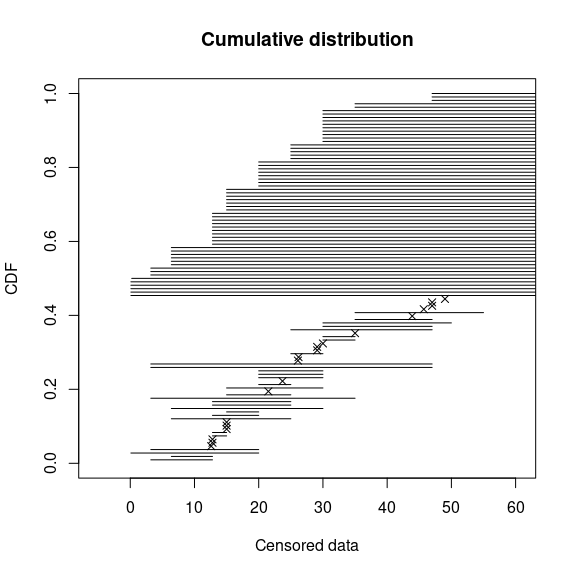

Simple plot of censored raw data (72-hour acute salinity tolerance of riverine macro-invertebrates from the salinity data set) as ordered points and intervals.

As for non censored data, one or more parametric distributions can be fitted to the censored data set, one at a time, but using in this case the fitdistcens function. This function estimates the vector of distribution parameters $\theta$ by maximizing the likelihood for censored data defined as:

$$\begin{equation} L(\theta) = \prod_{i=1}^{N_{nonC}} f(x_{i}|\theta)\times \prod_{j=1}^{N_{leftC}} F(x^{upper}_{j}|\theta) \\ \times \prod_{k=1}^{N_{rightC}} (1- F(x^{lower}_{k}|\theta))\times \prod_{m=1}^{N_{intC}} (F(x^{upper}_{m}|\theta)- F(x^{lower}_{j}|\theta))(\#eq:eq7) \end{equation}$$

with $x_{i}$ the $N_{nonC}$ non-censored observations, $x^{upper}_{j}$ upper values defining the $N_{leftC}$ left-censored observations, $x^{lower}_{k}$ lower values defining the $N_{rightC}$ right-censored observations, $[x^{lower}_{m} ; x^{upper}_{m}]$ the intervals defining the $N_{intC}$ interval-censored observations, and F the cumulative distribution function of the parametric distribution Helsel (2005).

As fitdist, fitdistcens returns the results of the fit of any parametric distribution to a data set as an S3 class object that can be easily printed, summarized or plotted. For the salinity data set, a lognormal distribution or a loglogistic can be fitted as commonly done in ecotoxicology for such data. As with fitdist, for some distributions (see Delignette-Muller et al. (2014) for details), it is necessary to specify initial values for the distribution parameters in the argument start. The plotdistcens function can help to find correct initial values for the distribution parameters in non trivial cases, by a manual iterative use if necessary.

fsal.ln <- fitdistcens(salinity, "lnorm")
fsal.ll <- fitdistcens(salinity, "llogis", start = list(shape = 5, scale = 40))
summary(fsal.ln)

## Fitting of the distribution ' lnorm ' By maximum likelihood on censored data 
## Parameters
##         estimate Std. Error
## meanlog   3.3854     0.6741
## sdlog     0.4961     0.5669
## Loglikelihood:  -139.1   AIC:  282.1   BIC:  287.5 
## Correlation matrix:
##         meanlog  sdlog
## meanlog  1.0000 0.2938
## sdlog    0.2938 1.0000

summary(fsal.ll)

## Fitting of the distribution ' llogis ' By maximum likelihood on censored data 
## Parameters
##       estimate Std. Error
## shape    3.421      4.321
## scale   29.930     20.210
## Loglikelihood:  -140.1   AIC:  284.1   BIC:  289.5 
## Correlation matrix:
##         shape   scale
## shape  1.0000 -0.2022
## scale -0.2022  1.0000

Computations of goodness-of-fit statistics have not yet been developed for fits using censored data but the quality of fit can be judged using Akaike and Schwarz’s Bayesian information criteria (AIC and BIC) and the goodness-of-fit CDF plot, respectively provided when summarizing or plotting an object of class fitdistcens. Functions cdfcompcens, qqcompcens and ppcompcens can also be used to compare the fit of various distributions to the same censored data set. Their calls are similar to the ones of cdfcomp, qqcomp and ppcomp. Below are examples of use of those functions with the two fitted distributions to the salinity data set (see Figure @ref(fig:cdfcompcens)). When qqcompcens and ppcompcens are used with more than one fitted distribution, the non uniqueness rectangles are not filled and a small noise is added on the y-axis in order to help the visualization of various fits. But we rather recommend the use of the plotstyle ggplot of qqcompcens and ppcompcens to compare the fits of various distributions as it provides a clearer plot splitted in facets (see ?graphcompcens).

par(mfrow = c(2, 2))
cdfcompcens(list(fsal.ln, fsal.ll), legendtext = c("lognormal", "loglogistic "))
qqcompcens(fsal.ln, legendtext = "lognormal")
ppcompcens(fsal.ln, legendtext = "lognormal")
qqcompcens(list(fsal.ln, fsal.ll), legendtext = c("lognormal", "loglogistic "),
           main = "Q-Q plot with 2 dist.")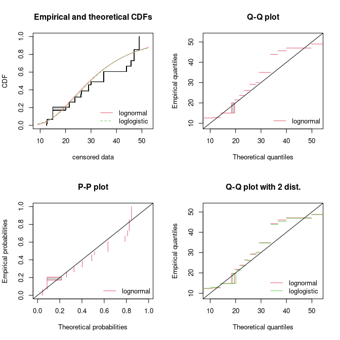

Some goodness-of-fit plots for fits of a lognormal and a loglogistic distribution to censored data: LC50 values from the salinity data set.

Function bootdistcens is the equivalent of bootdist for censored data, except that it only proposes nonparametric bootstrap. Indeed, it is not obvious to simulate censoring within a parametric bootstrap resampling procedure. The generic function quantile can also be applied to an object of class fitdistcens or bootdistcens, as for continuous non-censored data.

In addition to the fit of distributions to censored or non censored continuous data, our package can also accomodate discrete variables, such as count numbers, using the functions developped for continuous non-censored data. These functions will provide somewhat different graphs and statistics, taking into account the discrete nature of the modeled variable. The discrete nature of the variable is automatically recognized when a classical distribution is fitted to data (binomial, negative binomial, geometric, hypergeometric and Poisson distributions) but must be indicated by fixing argument discrete to TRUE in the call to functions in other cases. The toxocara data set included in the package corresponds to the observation of such a discrete variable. Numbers of Toxocara cati parasites present in digestive tract are reported from a random sampling of feral cats living on Kerguelen island (Fromont et al. 2001). We will use it to illustrate the case of discrete data.

data("toxocara")
str(toxocara)

## 'data.frame':    53 obs. of  1 variable:
##  $ number: int  0 0 0 0 0 0 0 0 0 0 ...

The fit of a discrete distribution to discrete data by maximum likelihood estimation requires the same procedure as for continuous non-censored data. As an example, using the toxocara data set, Poisson and negative binomial distributions can be easily fitted.

(ftoxo.P <- fitdist(toxocara$number, "pois"))

## Fitting of the distribution ' pois ' by maximum likelihood 
## Parameters:
##        estimate Std. Error
## lambda    8.679      2.946

(ftoxo.nb <- fitdist(toxocara$number, "nbinom"))

## Fitting of the distribution ' nbinom ' by maximum likelihood 
## Parameters:
##      estimate Std. Error
## size   0.3971     0.6035
## mu     8.6803    14.0871

For discrete distributions, the plot of an object of class fitdist simply provides two goodness-of-fit plots comparing empirical and theoretical distributions in density and in CDF. Functions cdfcomp and denscomp can also be used to compare several plots to the same data set, as follows for the previous fits (Figure @ref(fig:fittoxocarapoisnbinom)).

par(mfrow = c(1, 2))
denscomp(list(ftoxo.P, ftoxo.nb), legendtext = c("Poisson", "negative binomial"), fitlty = 1)
cdfcomp(list(ftoxo.P, ftoxo.nb), legendtext = c("Poisson", "negative binomial"), fitlty = 1)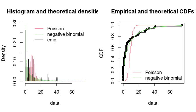

Comparison of the fits of a negative binomial and a Poisson distribution to numbers of Toxocara cati parasites from the toxocara data set.

When fitting discrete distributions, the Chi-squared statistic is computed by the gofstat function using cells defined by the argument chisqbreaks or cells automatically defined from the data in order to reach roughly the same number of observations per cell. This number is roughly equal to the argument meancount, or sligthly greater if there are some ties. The choice to define cells from the empirical distribution (data), and not from the theoretical distribution, was done to enable the comparison of Chi-squared values obtained with different distributions fitted on a same data set. If arguments chisqbreaks and meancount are both omitted, meancount is fixed in order to obtain roughly $(4n)^{2/5}$ cells, with $n$ the length of the data set (Vose 2010). Using this default option the two previous fits are compared as follows, giving the preference to the negative binomial distribution, from both Chi-squared statistics and information criteria:

gofstat(list(ftoxo.P, ftoxo.nb), fitnames = c("Poisson", "negative binomial"))

## Chi-squared statistic:  31257 7.486 
## Degree of freedom of the Chi-squared distribution:  5 4 
## Chi-squared p-value:  0 0.1123 
##    the p-value may be wrong with some theoretical counts < 5  
## Chi-squared table:
##       obscounts theo Poisson theo negative binomial
## <= 0         14     0.009014                 15.295
## <= 1          8     0.078237                  5.809
## <= 3          6     1.321767                  6.845
## <= 4          6     2.131298                  2.408
## <= 9          6    29.827829                  7.835
## <= 21         6    19.626223                  8.271
## > 21          7     0.005631                  6.537
## 
## Goodness-of-fit criteria
##                                Poisson negative binomial
## Akaike's Information Criterion    1017             322.7
## Bayesian Information Criterion    1019             326.6

4. Conclusion

The R package fitdistrplus allows to easily fit distributions. Our main objective while developing this package was to provide tools for helping R users to fit distributions to data. We have been encouraged to pursue our work by feedbacks from users of our package in various areas as food or environmental risk assessment, epidemiology, ecology, molecular biology, genomics, bioinformatics, hydraulics, mechanics, financial and actuarial mathematics or operations research. Indeed, this package is already used by a lot of practionners and academics for simple MLE fits Voigt et al. (2014), for MLE fits and goodness-of-fit statistics Vaninsky (2013), for MLE fits and bootstrap Rigaux et al. (2014), for MLE fits, bootstrap and goodness-of-fit statistics (Larras, Montuelle, and Bouchez 2013), for MME fit Sato et al. (2013), for censored MLE and bootstrap Contreras, Huerta, and Arnold (2013), for graphic analysing in (Anand, Yeturu, and Chandra 2012), for grouped-data fitting methods (Fu, Steiner, and Costafreda 2012) or more generally Drake, Chalabi, and Coker (2014).

The fitdistrplus package is complementary with the distrMod package (Kohl and Ruckdeschel 2010). distrMod provides an even more flexible way to estimate distribution parameters but its use requires a greater initial investment to learn how to manipulate the S4 classes and methods developed in the distr-family packages.

Many extensions of the fitdistrplus package are planned in the future: we target to extend to censored data some methods for the moment only available for non-censored data, especially concerning goodness-of-fit evaluation and fitting methods. We will also enlarge the choice of fitting methods for non-censored data, by proposing new goodness-of-fit distances (e.g., distances based on quantiles) for maximum goodness-of-fit estimation and new types of moments (e.g., limited expected values) for moment matching estimation. At last, we will consider the case of multivariate distribution fitting.

Acknowledgments

The package would not have been at this stage without the stimulating contribution of Régis Pouillot and Jean-Baptiste Denis, especially for its conceptualization. We also want to thank Régis Pouillot for his very valuable comments on the first version of this paper.

The authors gratefully acknowledges the two anonymous referees and the Editor for useful and constructive comments. The remaining errors, of course, should be attributed to the authors alone.

References

Anand, P., K. Yeturu, and N. Chandra. 2012. “PocketAnnotate: Towards Site-Based Function Annotation.” Nucleic Acids Research 40: 1–9.

Bagaria, A., V. Jaravine, Y. J. Huang, G. T. Montelione, and P. Güntert. 2012. “Protein Structure Validation by Generalized Linear Model Root-Mean-Square Deviation Prediction.” Protein Science 21 (2): 229–38.

Benavides-Piccione, R., I. Fernaud-Espinosa, V. Robles, R. Yuste, and J. DeFelipe. 2012. “Age-Based Comparison of Human Dendritic Spine Structure Using Complete Three-Dimensional Reconstructions.” Cerebral Cortex 23 (8): 1798–1810.

Blom, G. 1959. Statistical Estimates and Transformed Beta Variables. 1st ed. John Wiley & Sons.

Breitbach, N., K. Böhning-Gaese, I. Laube, and M. Schleuning. 2012. “Short Seed-Dispersal Distances and Low Seedling Recruitment in Farmland Populations of Bird-Dispersed Cherry Trees.” Journal of Ecology 100 (6): 1349–58.

Busschaert, P., A. H. Geeraerd, M. Uyttendaele, and J. F. VanImpe. 2010. “Estimating Distributions Out of Qualitative and (Semi)quantitative Microbiological Contamination Data for Use in Risk Assessment.” International Journal of Food Microbiology 138: 260–69.

Callau Poduje, Ana Claudia, Aslan Belli, and Uwe Haberlandt. 2013. “Dam Risk Assessment Based on Univariate Versus Bivariate Statistical Approaches - a Case Study for Argentina.” Hydrological Sciences Journal. https://doi.org/10.1080/02626667.2013.871014.

Casella, G., and R. L. Berger. 2002. Statistical Inference. 2nd ed. Duxbury Thomson Learning.

Commeau, N., E. Parent, M.-L. Delignette-Muller, and M. Cornu. 2012. “Fitting a Lognormal Distribution to Enumeration and Absence/Presence Data.” International Journal of Food Microbiology 155: 146–52.

Contreras, V. De La Huerta, H. Vaquera Huerta, and B. C. Arnold. 2013. “A Test for Equality of Variance with Censored Samples.” Journal of Statistical Computation and Simulation. https://doi.org/10.1080/00949655.2013.825095.

Croucher, N. J., S. R. Harris, L. Barquist, J. Parkhill, and S. D. Bentley. 2012. “A High-Resolution View of Genome-Wide Pneumococcal Transformation.” PLoS Pathogens 8 (6): e1002745.

Cullen, A. C., and H. C. Frey. 1999. Probabilistic Techniques in Exposure Assessment. 1st ed. Plenum Publishing Co.

D’Agostino, R. B., and M. A. Stephens. 1986. Goodness-of-Fit Techniques. 1st ed. Dekker.

Daelman, Jeff, Jeanne-Marie Membré, Liesbeth Jacxsens, An Vermeulen, Frank Devlieghere, and Mieke Uyttendaele. 2013. “A Quantitative Microbiological Exposure Assessment Model for Bacillus Cereus in REPFEDs.” International Journal of Food Microbiology 166 (3): 433–49.

Delignette-Muller, M. L., and M. Cornu. 2008. “Quantitative Risk Assessment for Escherichia Coli O157:H7 in Frozen Ground Beef Patties Consumed by Young Children in French Households.” International Journal of Food Microbiology 128 (1): 158–64. https://doi.org/https://doi.org/10.1016/j.ijfoodmicro.2008.05.040.

Delignette-Muller, M. L., R. Pouillot, J. B. Denis, and C. Dutang. 2014. : Help to Fit of a Parametric Distribution to Non-Censored or Censored Data. https://cran.r-project.org/package=fitdistrplus.

Drake, T., Z. Chalabi, and R. Coker. 2014. “Buy Now, saved Later? The Critical Impact of Time-to-Pandemic Uncertainty on Pandemic Cost-Effectiveness Analyses.” Health Policy and Planning. https://doi.org/10.1093/heapol/czt101.

Dutang, C., V. Goulet, and M. Pigeon. 2008. “: an R Package for Actuarial Science.” Journal of Statistical Software 25 (7): 1–37.

Efron, B., and R. J. Tibshirani. 1994. An Introduction to the Bootstrap. 1st ed. Chapman & Hall.

Eik, M., K. Luhmus, M. Tigasson, M. Listak, J. Puttonen, and H. Herrmann. 2013. “DC-Conductivity Testing Combined with Photometry for Measuring Fibre Orientations in SFRC.” Journal of Materials Science 48 (10): 3745–59.

Eling, M. 2012. “Fitting Insurance Claims to Skewed Distributions: Are the Skew-normal and the Skew-student Good Models?” Insurance: Mathematics and Economics 51 (2): 239–48.

Fiorelli, L. E., M. D. Ezcurra, E. M. Hechenleitner, E. Argañaraz, R. Jeremias, A. Taborda, M. J. Trotteyn, M. Belén von Baczko, and J. B. Desojo. 2013. “The Oldest Known Communal Latrines Provide Evidence of Gregarism in Triassic Megaherbivores.” Scientific Reports 3 (3348): 1–7.

Fromont, E, L Morvilliers, M Artois, and D Pontier. 2001. “Parasite Richness and Abundance in Insular and Mainland Feral Cats: Insularity or Density?” Parasitology 123 (Part 2): 143–51.

Fu, C. H. Y., H. Steiner, and S. G. Costafreda. 2012. “Predictive Neural Biomarkers of Clinical Response in Depression: A Meta-Analysis of Functional and Structural Neuroimaging Studies of Pharmacological and Psychological Therapies.” Neurobiology of Disease 52: 75–83.

González-Varo, J. P., J. V. López-Bao, and J. Guitián. 2012. “Functional Diversity Among Seed Dispersal Kernels Generated by Carnivorous Mammals.” Journal of Animal Ecology 82: 562–71.

Goulet, V. 2012. : An r Package for Actuarial Science. https://cran.r-project.org/package=actuar.

Guillier, Laurent, Corinne Danan, Hélène Bergis, Marie-Laure Delignette-Muller, Sophie Granier, Sylvie Rudelle, Annie Beaufort, and Anne Brisabois. 2013. “Use of Quantitative Microbial Risk Assessment when Investigating Foodborne Illness Outbreaks: the Example of a Monophasic Salmonella Typhimurium 4,5,12:i:- Outbreak Implicating Beef Burgers.” International Journal of Food Microbiology 166 (3): 471–78.

Helsel, D. R. 2005. Nondetects and Data Analysis: Statistics for Censored Environmental Data. 1st ed. John Wiley & Sons.

Hirano, S. S., M. K. Clayton, and C. D. Upper. 1994. “Estimation of and Temporal Changes in Means and Variances of Populations of Pseudomonas syringae on Snap Bean Leaflets.” Phytopathology 84 (9): 934–40.

Hoelzer, K., R. Pouillot, D. Gallagher, M. B. Silverman, J. Kause, and S. Dennis. 2012. “Estimation of Listeria Monocytogenes Transfer Coefficients and Efficacy of Bacterial Removal Through Cleaning and Sanitation.” International Journal of Food Microbiology 157 (2): 267–77.

Hose, G. C., and P. J. Van den Brink. 2004. “Confirming the Species-Sensitivity Distribution Concept for Endosulfan Using Laboratory, Mesocosm, and Field Data.” Archives of Environmental Contamination and Toxicology 47 (4): 511–20.

Hyndman, R. J., and Y. Fan. 1996. “Sample Quantiles in Statistical Packages.” The American Statistician 50: 361–65.

Jaloustre, S., M. Cornu, E. Morelli, V. Noel, and M. L. Delignette-Muller. 2011. “Bayesian Modeling of Clostridium perfringens Growth in Beef-in-Sauce Products.” Food Microbiology 28 (2): 311–20.

Jongenburger, I., M. W. Reij, E. P. J. Boer, M. H. Zwietering, and L. G. M. Gorris. 2012. “Modelling Homogeneous and Heterogeneous Microbial Contaminations in a Powdered Food Product.” International Journal of Food Microbiology 157 (1): 35–44.

Jordan, D. 2005. “Simulating the Sensitivity of Pooled-Sample Herd Tests for Fecal Salmonella in Cattle.” Preventive Veterinary Medicine 70 (1-2): 59–73.

Kefford, B. J., E. J. Fields, C. Clay, and D. Nugegoda. 2007. “Salinity Tolerance of Riverine Macroinvertebrates from the Southern Murray-Darling Basin.” Marine and Freshwater Research 58: 1019–31.

Klein, J. P., and M. L. Moeschberger. 2003. Survival Analysis: Techniques for Censored and Truncated Data. 2nd ed. Springer-Verlag.

Klugman, S. A., H. H. Panjer, and G. E. Willmot. 2009. Loss Models: From Data to Decisions. 3rd ed. John Wiley & Sons.

Koch, F. H., D. Yemshanov, R. D. Magarey, and W. D. Smith. 2012. “Dispersal of Invasive Forest Insects via Recreational Firewood: A Quantitative Analysis.” Journal of Economic Entomology 105 (2): 438–50.

Kohl, M., and P. Ruckdeschel. 2010. “R Package : S4 Classes and Methods for Probability Models.” Journal of Statistical Software 35 (10): 1–27.

Larras, Floriane, Bernard Montuelle, and Agnès Bouchez. 2013. “Assessment of Toxicity Thresholds in Aquatic Environments: Does Benthic Growth of Diatoms Affect their Exposure and Sensitivity to Herbicides?” Science of The Total Environment 463-464: 469–77.

Leha, A., T. Beissbarth, and K. Jung. 2011. “Sequential Interim Analyses of Survival Data in DNA Microarray Experiments.” BMC Bioinformatics 12 (127): 1–14.

Luangkesorn, K. L., B. A. Norman, Y. Zhuang, M. Falbo, and J. Sysko. 2012. “Practice Summaries: Designing Disease Prevention and Screening Centers in Abu Dhabi.” Interfaces 42 (4): 406–9.

Luceno, A. 2006. “Fitting the Generalized Pareto Distribution to Data Using Maximum Goodness-of-fit Estimators.” Computational Statistics and Data Analysis 51 (2): 904–17.

Malá, I. 2013. “The Use of Finite Mixtures of Lognormal and Gamma Distributions.” Research Journal of Economics, Business and ICT 8 (2): 55–61.

Mandl, J. N., J. P. Monteiro, N. Vrisekoop, and R. N. Germain. 2013. “T Cell-Positive Selection Uses Self-Ligand Binding Strength to Optimize Repertoire Recognition of Foreign Antigens.” Immunity 38 (2): 263–74.

Marquetoux, N., M. Paul, S. Wongnarkpet, C. Poolkhet, W. Thanapongtham, F. Roger, C. Ducrot, and K. Chalvet-Monfray. 2012. “Estimating Spatial and Temporal Variations of the Reproduction Number for Highly Pathogenic Avian Influenza H5N1 Epidemic in Thailand.” Preventive Veterinary Medicine 106 (2): 143–51.

McNeil, A. J. 1997. “Estimating the Tails of Loss Severity Distributions Using Extreme Value Theory.” ASTIN Bulletin 27 (1): 117–37.

Méheust, D., P. Le Cann, T. Reponen, J. Wakefield, and S. Vesper. 2012. “Possible Application of the Environmental Relative Moldiness Index in France: a Pilot Study in Brittany.” International Journal of Hygiene and Environmental Health 216 (3): 333–40.

Meyer, W. K., S. Zhang, S. Hayakawa, H. Imai, and M. Przeworski. 2013. “The Convergent Evolution of Blue Iris Pigmentation in Primates Took Distinct Molecular Paths.” American Journal of Physical Anthropology 151 (3): 398–407.

Nadarajah, S., and S. A. A. Bakar. 2013. “CompLognormal: An R Package for Composite Lognormal Distributions.” R Journal 5 (2): 98–104.

Orellano, P. W., J. I. Reynoso, A. Grassi, A. Palmieri, O. Uez, and O. Carlino. 2012. “Estimation of the Serial Interval for Pandemic Influenza (pH1N1) in the Most Southern Province of Argentina.” Iranian Journal of Public Health 41 (12): 26–29.

Posthuma, L., G. W. Suter, and T. P. Traas. 2010. Species Sensitivity Distributions in Ecotoxicology. Environmental and Ecological Risk Assessment Series. Taylor & Francis.

Pouillot, R., and M. L. Delignette-Muller. 2010. “Evaluating Variability and Uncertainty Separately in Microbial Quantitative Risk Assessment using two R Packages.” International Journal of Food Microbiology 142 (3): 330–40.

Pouillot, R., M. L. Delignette-Muller, and J. B. Denis. 2011. : Tools for Two-Dimensional Monte-Carlo Simulations. https://cran.r-project.org/package=mc2d.

Pouillot, R., K. Hoelzer, Y. Chen, and S. Dennis. 2012. “Estimating Probability Distributions of Bacterial Concentrations in Food Based on Data Generated Using the Most Probable Number (MPN) Method for Use in Risk Assessment.” Food Control 29 (2): 350–57.

Prosser, D. J., L. L. Hungerford, R. M. Erwin, M. A. Ottinger, J. Y. Takekawa, and E. C. Ellis. 2013. “Mapping Avian Influenza Transmission Risk at the Interface of Domestic Poultry and Wild Birds.” Frontiers in Public Health 1 (28): 1–11.

R Development Core Team. 2013. R: A Language and Environment for Statistical Computing. Vienna, Austria. https://www.r-project.org/.

Ricci, V. 2005. “Fitting Distributions with r.” https://cran.r-project.org/doc/contrib/Ricci-distributions-en.pdf.

Rigaux, Clémence, Stéphane André, Isabelle Albert, and Frédéric Carlin. 2014. “Quantitative Assessment of the Risk of Microbial Spoilage in Foods. Prediction of Non-Stability at 55$\,^{\circ}$c Caused by Geobacillus Stearothermophilus in Canned Green Beans.” International Journal of Food Microbiology 171: 119–28.

Sak, H., and C. Haksoz. 2011. “A Copula-Based Simulation Model for Supply Portfolio Risk.” Journal of Operational Risk 6 (3): 15–38.

Samuel-Rosa, A., R. Simao Diniz Dalmolin, and P. Miguel. 2013. “Building Predictive Models of Soil Particle-Size Distribution.” Revista Brasileira de Ciencia Do Solo 37: 422–30.

Sato, Maria Ines Z., Ana Tereza Galvani, Jose Antonio Padula, Adelaide Cassia Nardocci, Marcelo de Souza Lauretto, Maria Tereza Pepe Razzolini, and Elayse Maria Hachich. 2013. “Assessing the Infection Risk of Giardia and Cryptosporidium in Public Drinking Water Delivered by Surface Water Systems in Sao Paulo State, Brazil.” Science of The Total Environment 442: 389–96.

Scholl, C. F., C. C. Nice, J. A. Fordyce, Z. Gompert, and M. L. Forister. 2012. “Larval Performance in the Context of Ecological Diversification and Speciation in Lycaeides Butterflies.” International Journal of Ecology 2012 (ID 242154): 1–13.

Simó, J., Francesc Casaña, and J. Sabaté. 2013. “Modelling ‘calçots’ (Alium cepa L.) Growth by Gompertz Function.” Statistics and Operations Research Transactions 37 (1): 95–106.

Srinivasan, S., T. P. Sorrell, J. P. Brooks, D. J. Edwards, and R. Diehl McDougle. 2013. “Workforce Assessment Method for an Urban Police Department: Using Analytics to Estimate Patrol Staffing.” Policing: An International Journal of Police Strategies & Management 36 (4): 702–18.

Stagge, J. H., and G. E. Moglen. 2013. “A Nonparametric Stochastic Method for Generating Daily Climate-Adjusted Streamflows.” Water Resources Research 49 (10): 6179–93.

Suuronen, J. P., A. Kallonen, M. Eik, J. Puttonen, Ritva Serimaa, and Heiko Herrmann. 2012. “Analysis of Short Fibres Orientation in Steel Fibre-Reinforced Concrete (SFRC) by x-Ray Tomography.” Journal of Materials Science 48 (3): 1358–67.

Tarnczi, T., V. Fenyves, and Z. Bcs. 2011. “The Business Uncertainty and Variability Management with Real Options Models Combined Two Dimensional Simulation.” International Journal of Management Cases 13 (3): 159–67.

Tello, A., B. Austin, and T. C. Telfer. 2012. “Selective Pressure of Antibiotic Pollution on Bacteria of Importance to Public Health.” Environmental Health Perspectives 120 (8): 1100–1106.

Therneau, T. 2011. : Survival Analysis, Including Penalized Likelihood. https://cran.r-project.org/package=survival.

Tikole, S., V. Jaravine, V. Yu Orekhov, and P. Guentert. 2013. “Effects of NMR spectral resolution on protein structure calculation.” PloS One 8 (7): e68567.

Tse, Y. K. 2009. Nonlife Actuarial Models: Theory, Methods and Evaluation. 1st ed. International Series on Actuarial Science. Cambridge University Press.

Turnbull, B. W. 1974. “Nonparametric Estimation of a Survivorship Function with Doubly Censored Data.” Journal of the American Statistical Association 69 (345): 169–73.

Vaninsky, A. Y. 2013. “Stochastic DEA with a Perfect Object and Its Application to Analysis of Environmental Efficiency.” American Journal of Applied Mathematics and Statistics 1 (4): 57–63.

Venables, W. N., and B. D. Ripley. 2010. Modern Applied Statistics with S. 4th ed. Springer-Verlag.

Viana, D. S., L. Santamará, T. C. Michot, and J. Figuerola. 2013. “Allometric Scaling of Long-Distance Seed Dispersal by Migratory Birds.” The American Naturalist 181 (5): 649–62.

Voigt, Christian C., Linn S. Lehnert, Ana G. Popa-Lisseanu, Mateusz Ciechanowski, Péter Estók, Florian Gloza-Rausch, Tamás Goerfoel, et al. 2014. “The Trans-Boundary Importance of Artificial Bat hibernacula in Managed European Forests.” Biodiversity and Conservation 23: 617–31.

Vose, D. 2010. Quantitative Risk Analysis. A Guide to Monte Carlo Simulation Modelling. 1st ed. John Wiley & Sons.

Wang, Yong. 2007. “On Fast Computation of the Non-Parametric Maximum Likelihood Estimate of a Mixing Distribution.” Journal of the Royal Statistical Society: Series B (Statistical Methodology) 69 (2): 185–98.

———. 2008. “Dimension-Reduced Nonparametric Maximum Likelihood Computation for Interval-Censored Data.” Computational Statistics & Data Analysis 52 (5): 2388–2402.

Wang, Yong, and Shabnam Fani. 2018. “Nonparametric Maximum Likelihood Computation of a u-Shaped Hazard Function.” Statistics and Computing 28 (1): 187–200.

Wang, Yong, and Stephen M Taylor. 2013. “Efficient Computation of Nonparametric Survival Functions via a Hierarchical Mixture Formulation.” Statistics and Computing 23 (6): 713–25.

Wayland, M. T. 2013. “Morphological Variation in Echinorhynchus truttae Schrank, 1788 and the Echinorhynchus bothniensis Zdzitowiecki & Valtonen, 1987 species complex from freshwater fishes of northern Europe.” Biodiversity Data Journal 1: e975.

Westphal-Fitch, G., and W. T. Fitch. 2013. “Spatial Analysis of ‘Crazy Quilts,’ a Class of Potentially Random Aesthetic Artefacts.” PloS One 8 (9): e74055.

Wu, Xing Zheng. 2013a. “Probabilistic Slope Stability Analysis by a Copula-Based Sampling Method.” Computational Geosciences 17 (5): 739–55.

———. 2013b. “Trivariate Analysis of Soil Ranking-Correlated Characteristics and Its Application to Probabilistic Stability Assessments in Geotechnical Engineering Problems.” Soils and Foundations 53 (4): 540–56.

Zhang, Yu, Emad Habib, Robert J. Kuligowski, and Dongsoo Kim. 2013. “Joint Distribution of Multiplicative Errors in Radar and Satellite {QPEs} and Its Use in Estimating the Conditional Exceedance Probability.” Advances in Water Resources 59: 133–45.