Plot of empirical and theoretical distributions for non-censored data

Plots an empirical distribution (non-censored data) with a theoretical one if specified.

Usage

plotdist(data, distr, para, histo = TRUE, breaks = "default", 
  demp = FALSE, discrete, ...)

Arguments

data: A numeric vector.
distr: A character string "name" naming a distribution for which the corresponding density function dname, the corresponding distribution function pname and the corresponding quantile function qname must be defined, or directly the density function. This argument may be omitted only if para is omitted.
para: A named list giving the parameters of the named distribution. This argument may be omitted only if distr is omitted.
histo: A logical to plot the histogram using the hist function.
breaks: If "default" the histogram is plotted with the function hist with its default breaks definition. Else breaks is passed to the function hist. This argument is not taken into account if discrete is TRUE.
demp: A logical to plot the empirical density on the first plot (alone or superimposed on the histogram depending of the value of the argument histo) using the density function.
discrete: If TRUE, the distribution is considered as discrete. If both distr and discrete are missing, discrete is set to FALSE. If discrete is missing but not distr, discrete is set to TRUE when distr belongs to "binom", "nbinom","geom", "hyper" or "pois".
...: further graphical arguments passed to graphical functions used in plotdist.

Details

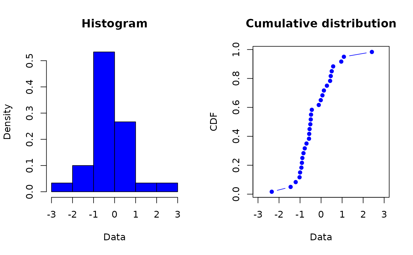
Empirical and, if specified, theoretical distributions are plotted in density and in cdf. For the plot in density, the user can use the arguments histo and demp to specify if he wants the histogram using the function hist, the density plot using the function density, or both (at least one of the two arguments must be put to "TRUE"). For continuous distributions, the function hist is used with its default breaks definition if breaks is "default" or passing breaks as an argument if it differs from "default". For continuous distribution and when a theoretical distribution is specified by both arguments distname and para, Q-Q plot (plot of the quantiles of the theoretical fitted distribution (x-axis) against the empirical quantiles of the data) and P-P plot (i.e. for each value of the data set, plot of the cumulative density function of the fitted distribution (x-axis) against the empirical cumulative density function (y-axis)) are also given (Cullen and Frey, 1999). The function ppoints (with default parameter for argument a) is used for the Q-Q plot, to generate the set of probabilities at which to evaluate the inverse distribution. NOTE THAT FROM VERSION 0.4-3, ppoints is also used for P-P plot and cdf plot for continuous data. To personalize the four plots proposed for continuous data, for example to change the plotting position, we recommend the use of functions cdfcomp, denscomp, qqcomp and ppcomp.

References

Cullen AC and Frey HC (1999), Probabilistic techniques in exposure assessment. Plenum Press, USA, pp. 81-155.

Delignette-Muller ML and Dutang C (2015), fitdistrplus: An R Package for Fitting Distributions. Journal of Statistical Software, 64(4), 1-34, doi:10.18637/jss.v064.i04 .

Author

Marie-Laure Delignette-Muller and Christophe Dutang.

Examples

# (1) Plot of an empirical distribution with changing 
# of default line types for CDF and colors
# and optionally adding a density line
#
set.seed(1234)
x1 <- rnorm(n=30)
plotdist(x1)

plotdist(x1,demp = TRUE)

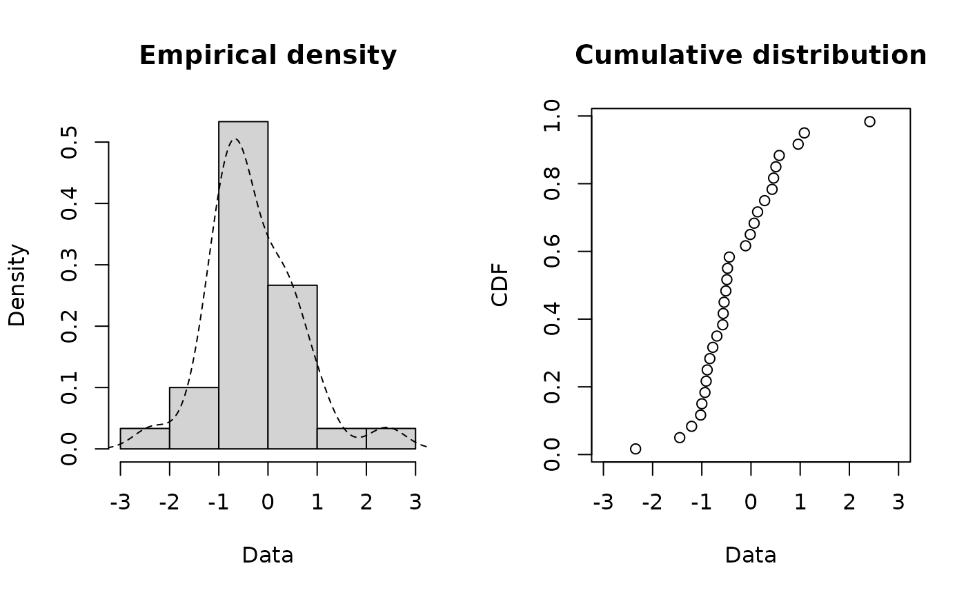plotdist(x1,histo = FALSE, demp = TRUE)
#> Warning: arguments ‘freq’, ‘main’, ‘xlab’ are not made use of

plotdist(x1, col="blue", type="b", pch=16)
#> Warning: graphical parameter "type" is obsolete
#> Warning: graphical parameter "type" is obsolete
#> Warning: graphical parameter "type" is obsolete
#> Warning: graphical parameter "type" is obsolete

plotdist(x1, type="s")
#> Warning: graphical parameter "type" is obsolete
#> Warning: graphical parameter "type" is obsolete
#> Warning: graphical parameter "type" is obsolete
#> Warning: graphical parameter "type" is obsolete


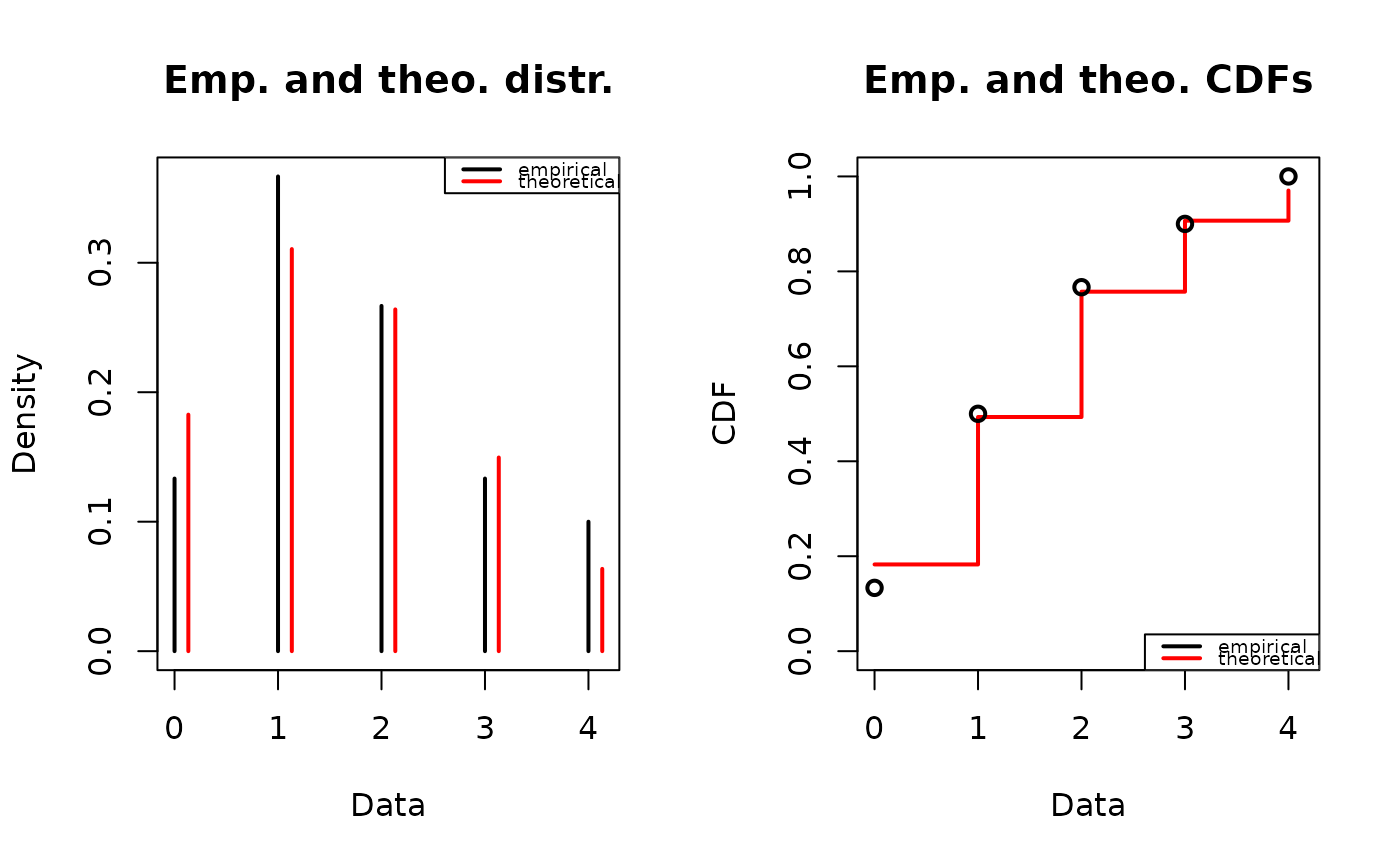
# (2) Plot of a discrete distribution against data
#
set.seed(1234)
x2 <- rpois(n=30, lambda = 2)
plotdist(x2, discrete=TRUE)

plotdist(x2, "pois", para=list(lambda = mean(x2)))

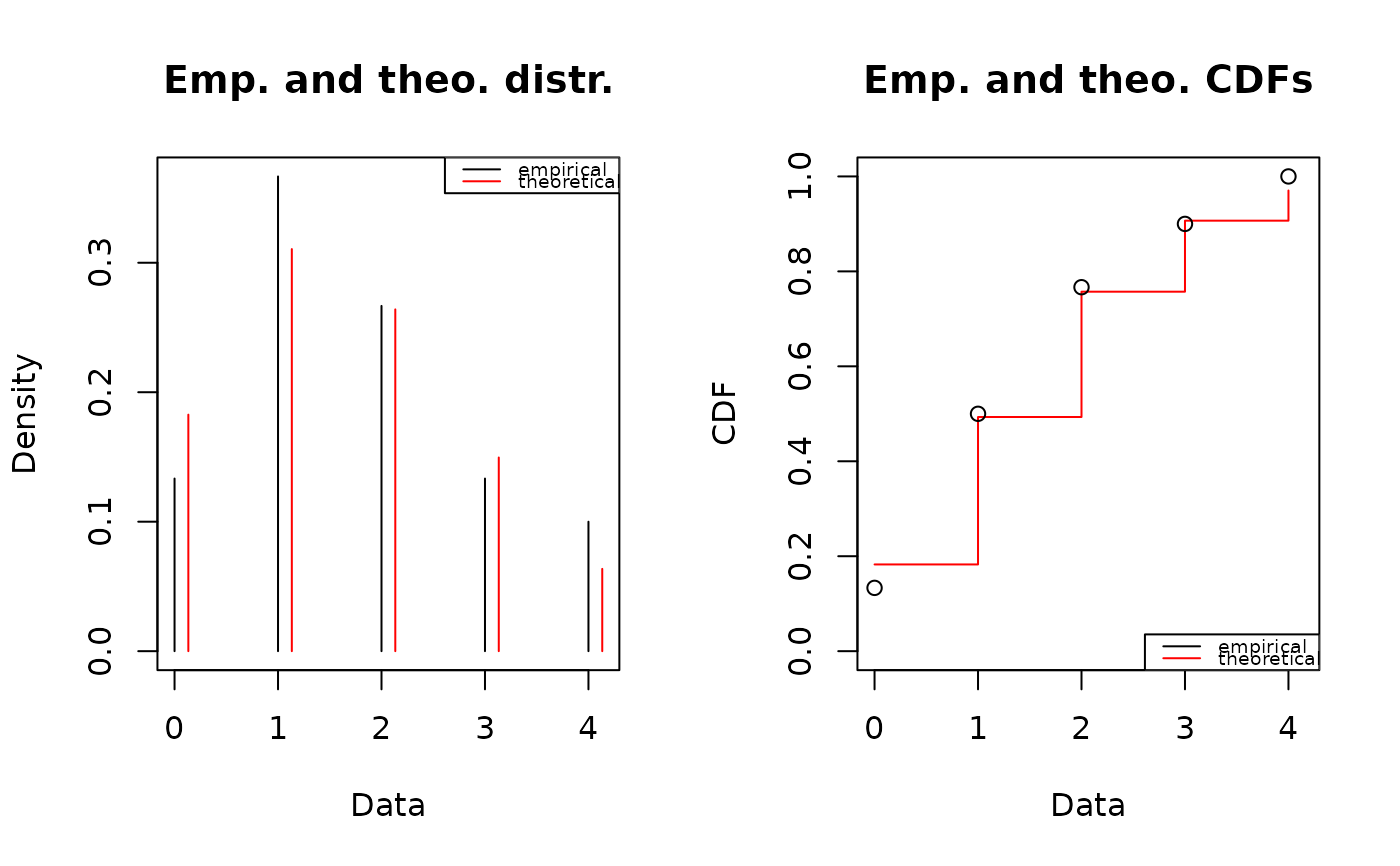plotdist(x2, "pois", para=list(lambda = mean(x2)), lwd="2")


# (3) Plot of a continuous distribution against data
#
xn <- rnorm(n=100, mean=10, sd=5)
plotdist(xn, "norm", para=list(mean=mean(xn), sd=sd(xn)))

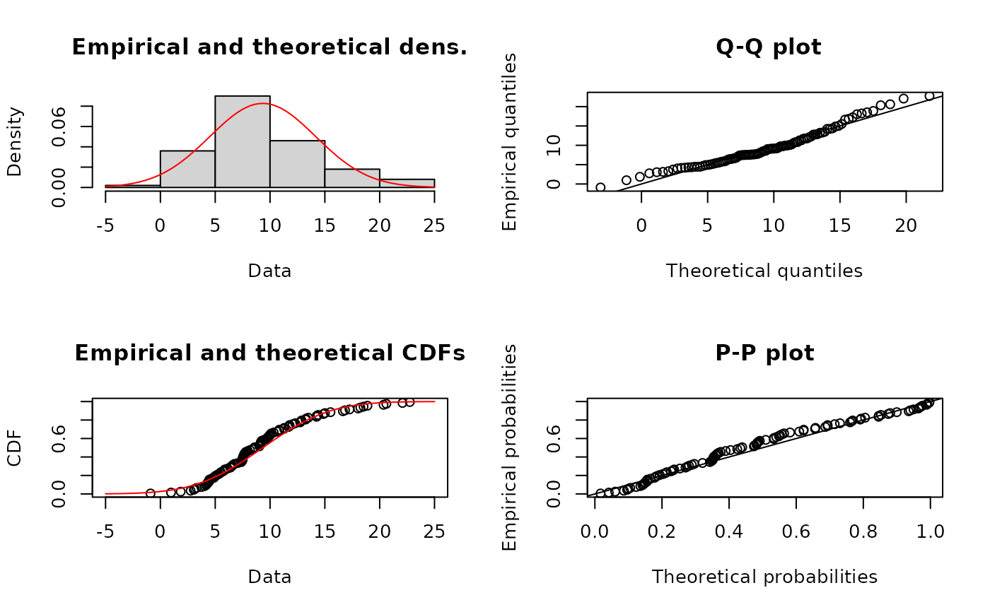plotdist(xn, "norm", para=list(mean=mean(xn), sd=sd(xn)), pch=16)

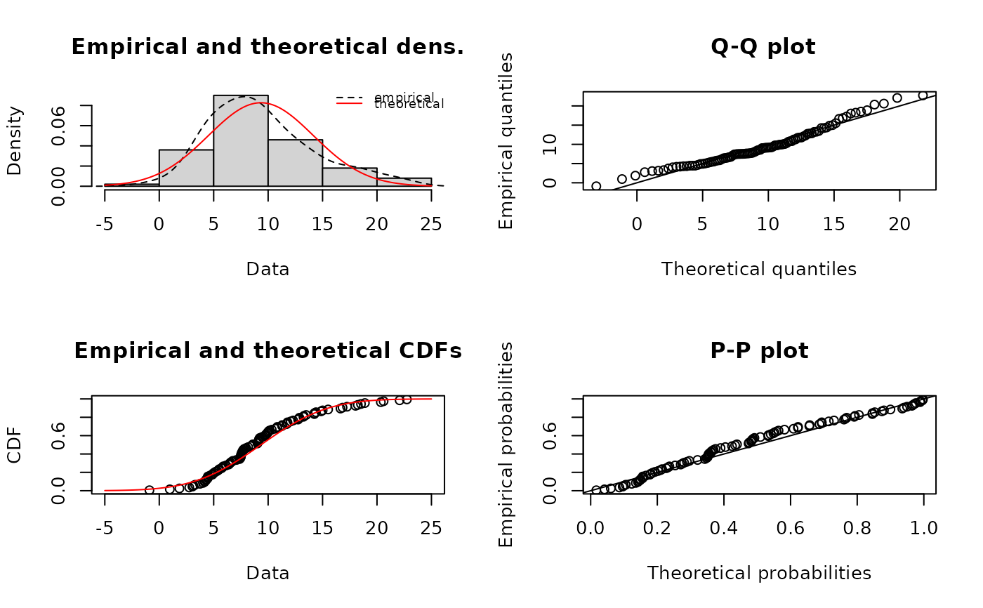
plotdist(xn, "norm", para=list(mean=mean(xn), sd=sd(xn)), demp = TRUE)

plotdist(xn, "norm", para=list(mean=mean(xn), sd=sd(xn)), 
histo = FALSE, demp = TRUE)


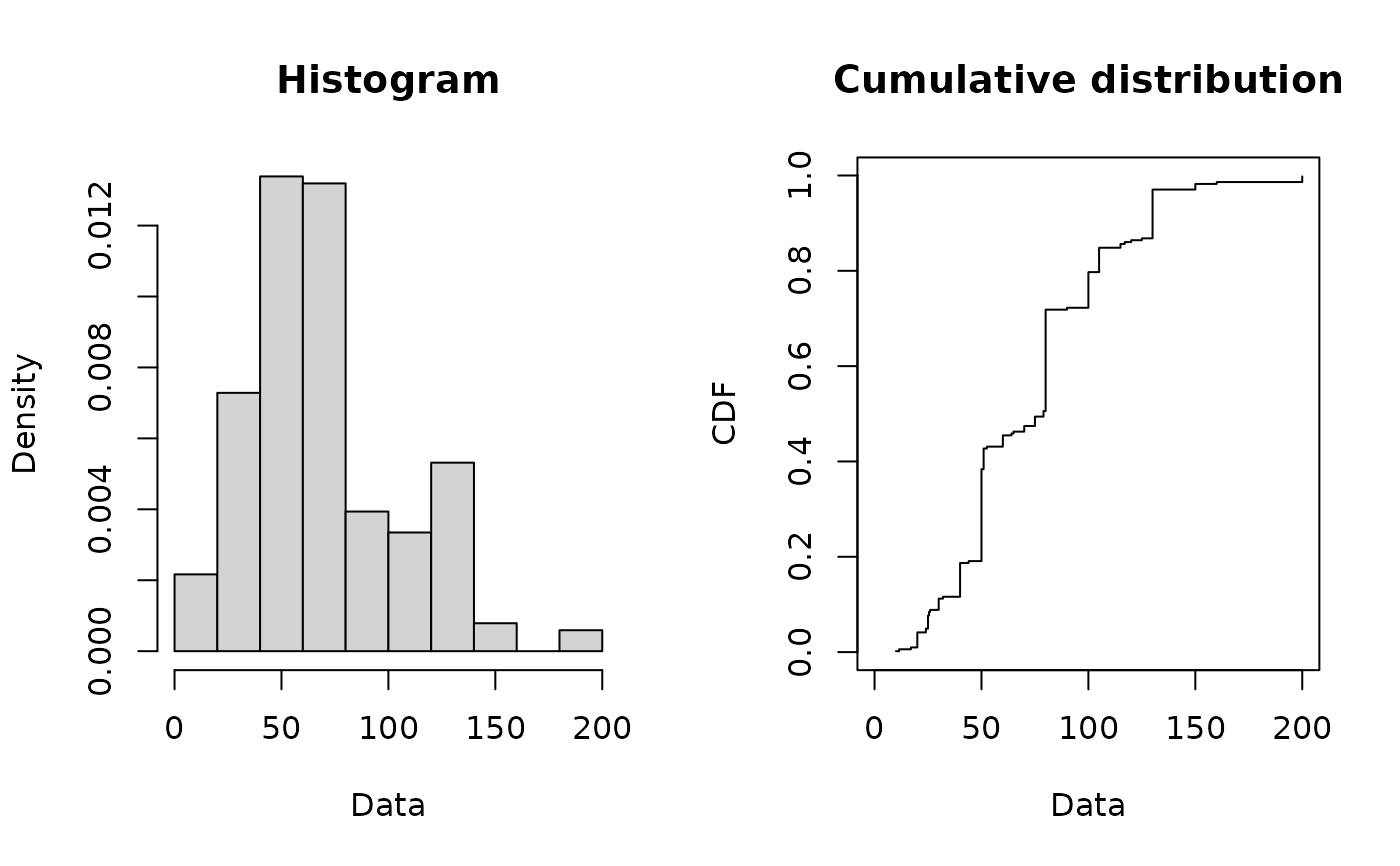
# (4) Plot of serving size data
#
data(groundbeef)
plotdist(groundbeef$serving, type="s")
#> Warning: graphical parameter "type" is obsolete
#> Warning: graphical parameter "type" is obsolete
#> Warning: graphical parameter "type" is obsolete
#> Warning: graphical parameter "type" is obsolete


# (5) Plot of numbers of parasites with a Poisson distribution 
data(toxocara)
number <- toxocara$number
plotdist(number, discrete = TRUE)

plotdist(number,"pois",para=list(lambda=mean(number)))