Description of an empirical distribution for non-censored data

Computes descriptive parameters of an empirical distribution for non-censored data and provides a skewness-kurtosis plot.

Usage

descdist(data, discrete = FALSE, boot = NULL, method = "unbiased",
graph = TRUE, print = TRUE, obs.col = "red", obs.pch = 16, boot.col = "orange")

# S3 method for class 'descdist'
print(x, ...)

Arguments

data: A numeric vector.
discrete: If TRUE, the distribution is considered as discrete.
boot: If not NULL, boot values of skewness and kurtosis are plotted from bootstrap samples of data. boot must be fixed in this case to an integer above 10.
method: "unbiased" for unbiased estimated values of statistics or "sample" for sample values.
graph: If FALSE, the skewness-kurtosis graph is not plotted.
print: If FALSE, the descriptive parameters computed are not printed.
obs.col: Color used for the observed point on the skewness-kurtosis graph.
obs.pch: plotting character used for the observed point on the skewness-kurtosis graph.
boot.col: Color used for bootstrap sample of points on the skewness-kurtosis graph.
x: An object of class "descdist".
...: Further arguments to be passed to generic functions

Details

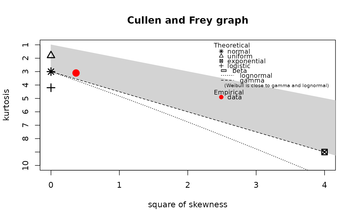
Minimum, maximum, median, mean, sample sd, and sample (if method=="sample") or by default unbiased estimations of skewness and Pearsons's kurtosis values are printed (Sokal and Rohlf, 1995). A skewness-kurtosis plot such as the one proposed by Cullen and Frey (1999) is given for the empirical distribution. On this plot, values for common distributions are also displayed as a tools to help the choice of distributions to fit to data. For some distributions (normal, uniform, logistic, exponential for example), there is only one possible value for the skewness and the kurtosis (for a normal distribution for example, skewness = 0 and kurtosis = 3), and the distribution is thus represented by a point on the plot. For other distributions, areas of possible values are represented, consisting in lines (gamma and lognormal distributions for example), or larger areas (beta distribution for example). The Weibull distribution is not represented on the graph but it is indicated on the legend that shapes close to lognormal and gamma distributions may be obtained with this distribution.

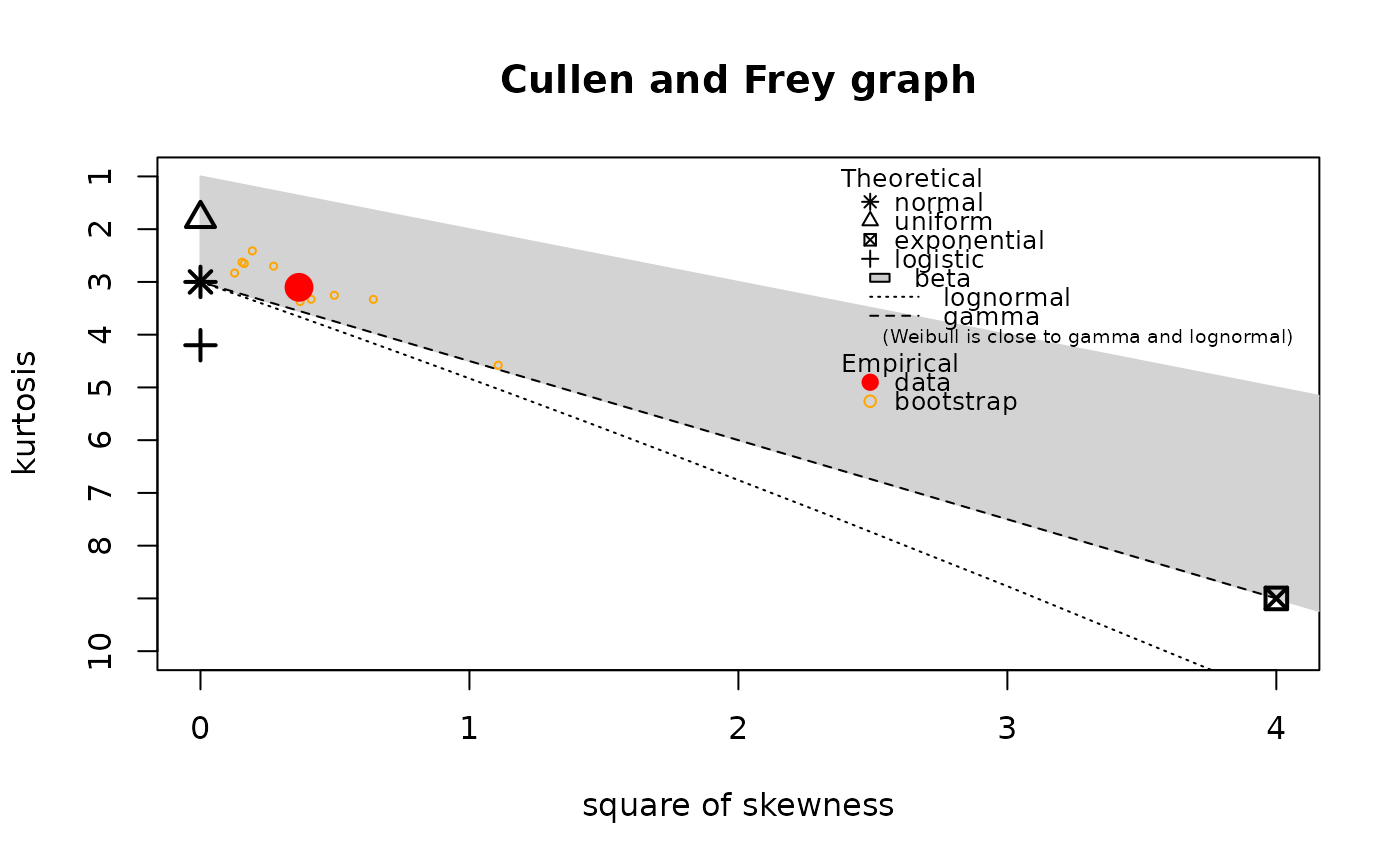
In order to take into account the uncertainty of the estimated values of kurtosis and skewness from data, the data set may be bootstraped by fixing the argument boot to an integer above 10. boot values of skewness and kurtosis corresponding to the boot bootstrap samples are then computed and reported in blue color on the skewness-kurtosis plot.

If discrete is TRUE, the represented distributions are the Poisson, negative binomial distributions, and the normal distribution to which previous discrete distributions may converge. If discrete is FALSE, these are uniform, normal, logistic, lognormal, beta and gamma distributions.

Value

descdist returns a list with 7 components,

min: the minimum value
max: the maximum value
median: the median value
mean: the mean value
sd: the standard deviation sample or estimated value
skewness: the skewness sample or estimated value
kurtosis: the kurtosis sample or estimated value
method: the method specified in input ("unbiased" for unbiased estimated values of statistics or "sample" for sample values.

References

Cullen AC and Frey HC (1999), Probabilistic techniques in exposure assessment. Plenum Press, USA, pp. 81-159.

Evans M, Hastings N and Peacock B (2000), Statistical distributions. John Wiley and Sons Inc, doi:10.1002/9780470627242 .

Sokal RR and Rohlf FJ (1995), Biometry. W.H. Freeman and Company, USA, pp. 111-115.

Delignette-Muller ML and Dutang C (2015), fitdistrplus: An R Package for Fitting Distributions. Journal of Statistical Software, 64(4), 1-34, doi:10.18637/jss.v064.i04 .

Author

Marie-Laure Delignette-Muller and Christophe Dutang.

Examples

# (1) Description of a sample from a normal distribution
# with and without uncertainty on skewness and kurtosis estimated by bootstrap 
#
set.seed(1234)
x1 <- rnorm(100)
descdist(x1)

#> summary statistics
#> ------
#> min:  -2.345698   max:  2.548991 
#> median:  -0.384628 
#> mean:  -0.1567617 
#> estimated sd:  1.004405 
#> estimated skewness:  0.6052442 
#> estimated kurtosis:  3.102441 
descdist(x1,boot=11)

#> summary statistics
#> ------
#> min:  -2.345698   max:  2.548991 
#> median:  -0.384628 
#> mean:  -0.1567617 
#> estimated sd:  1.004405 
#> estimated skewness:  0.6052442 
#> estimated kurtosis:  3.102441 

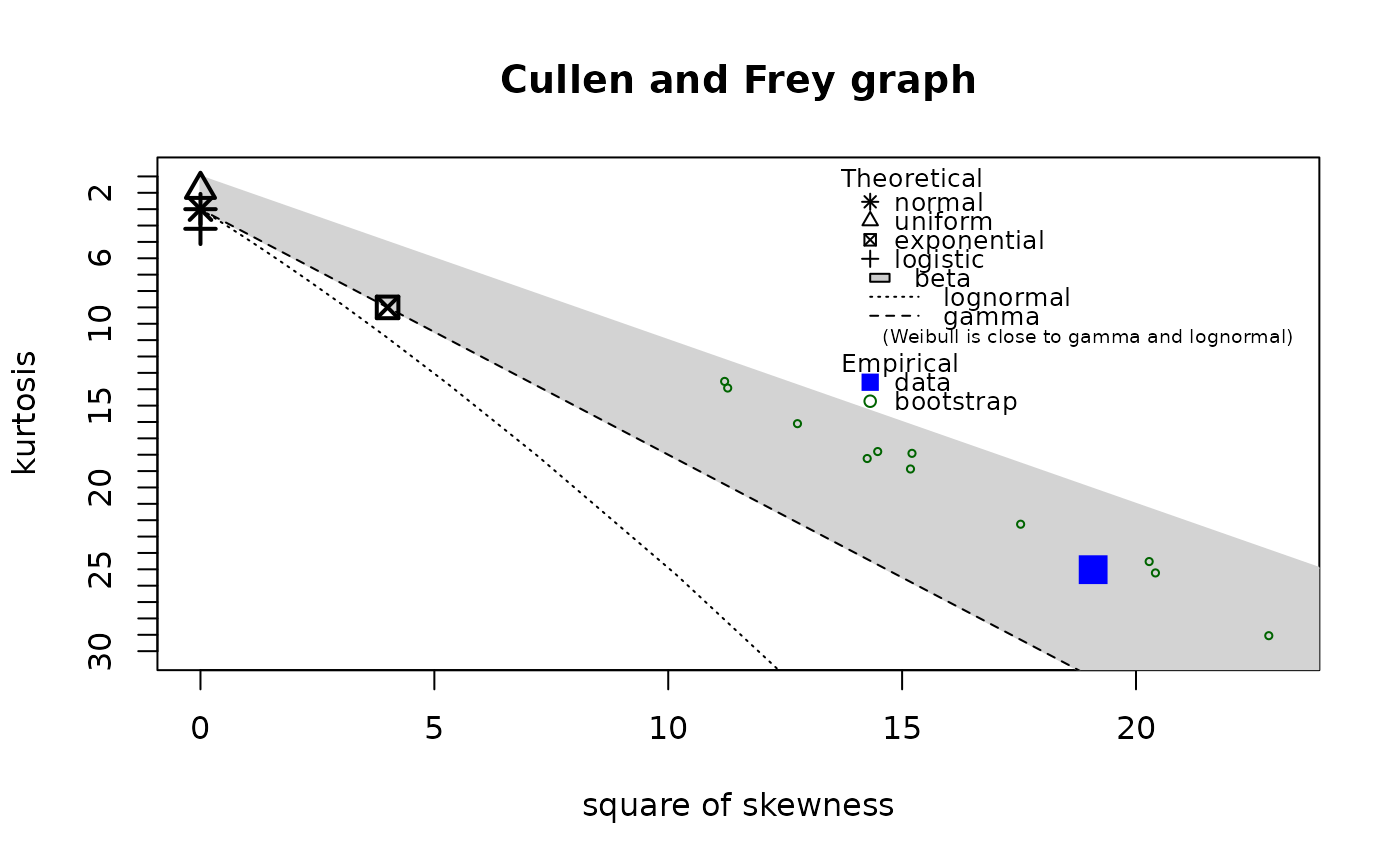
# (2) Description of a sample from a beta distribution
# with uncertainty on skewness and kurtosis estimated by bootstrap
# with changing of default colors and plotting character for observed point
#
descdist(rbeta(100,shape1=0.05,shape2=1),boot=11,
 obs.col="blue", obs.pch = 15, boot.col="darkgreen")

#> summary statistics
#> ------
#> min:  3.937372e-36   max:  0.8890347 
#> median:  5.660314e-06 
#> mean:  0.04094397 
#> estimated sd:  0.1281058 
#> estimated skewness:  4.368522 
#> estimated kurtosis:  25.02241 

# (3) Description of a sample from a gamma distribution
# with uncertainty on skewness and kurtosis estimated by bootstrap
# without plotting 
#
descdist(rgamma(100,shape=2,rate=1),boot=11,graph=FALSE)
#> summary statistics
#> ------
#> min:  0.0753002   max:  8.631328 
#> median:  1.627968 
#> mean:  1.989657 
#> estimated sd:  1.443636 
#> estimated skewness:  1.509842 
#> estimated kurtosis:  6.691933 

# (4) Description of a sample from a Poisson distribution
# with uncertainty on skewness and kurtosis estimated by bootstrap 
#
descdist(rpois(100,lambda=2),discrete=TRUE,boot=11)

#> summary statistics
#> ------
#> min:  0   max:  6 
#> median:  2 
#> mean:  1.98 
#> estimated sd:  1.377892 
#> estimated skewness:  0.5802731 
#> estimated kurtosis:  3.037067 

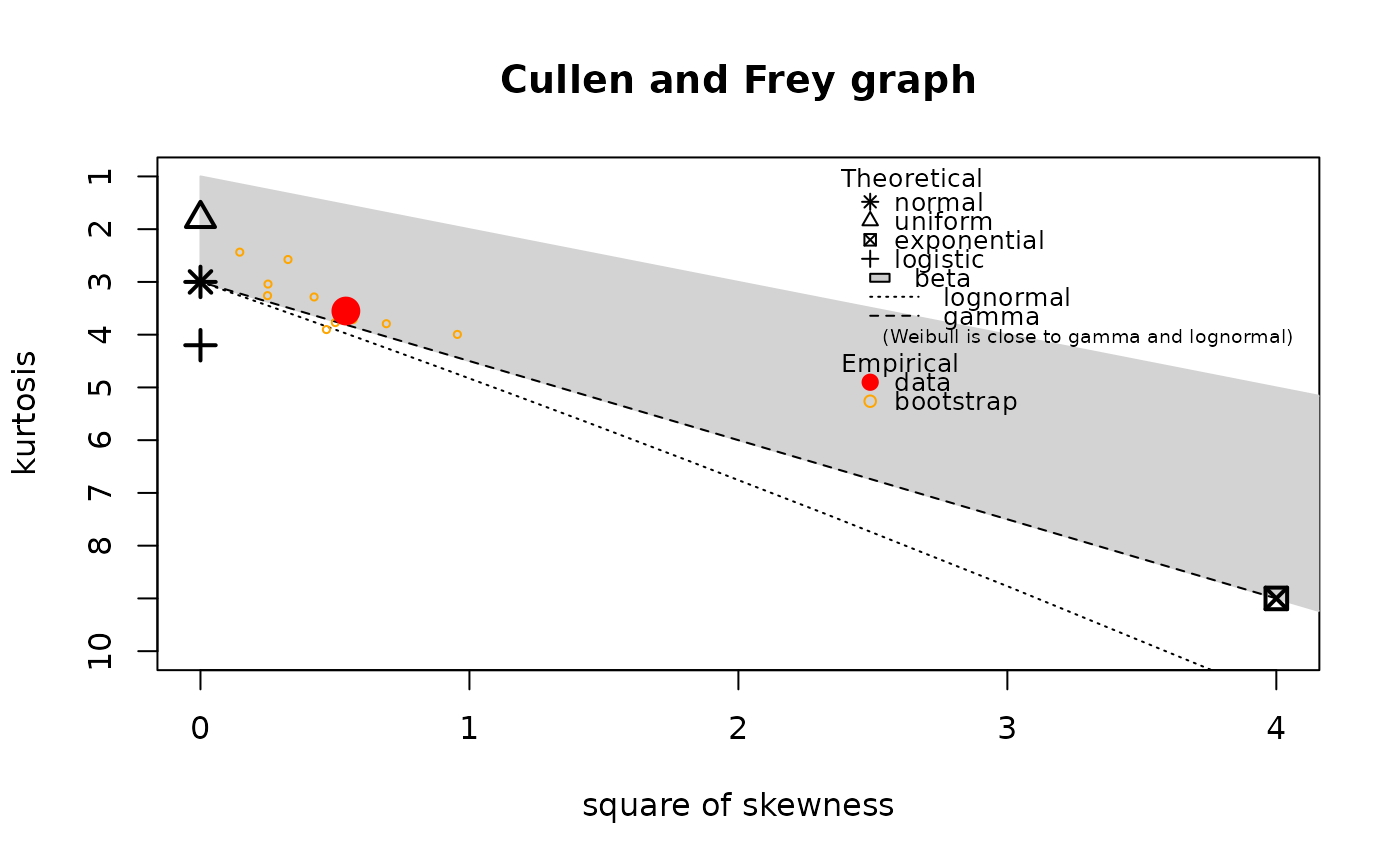
# (5) Description of serving size data
# with uncertainty on skewness and kurtosis estimated by bootstrap 
#
data(groundbeef)
serving <- groundbeef$serving
descdist(serving, boot=11)

#> summary statistics
#> ------
#> min:  10   max:  200 
#> median:  79 
#> mean:  73.64567 
#> estimated sd:  35.88487 
#> estimated skewness:  0.7352745 
#> estimated kurtosis:  3.551384