Graphical comparison of multiple fitted distributions (for non-censored data)

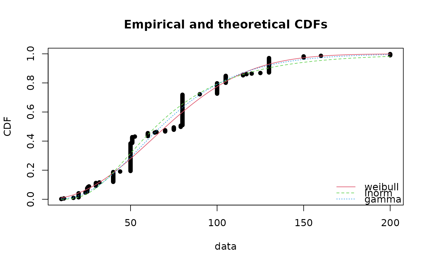
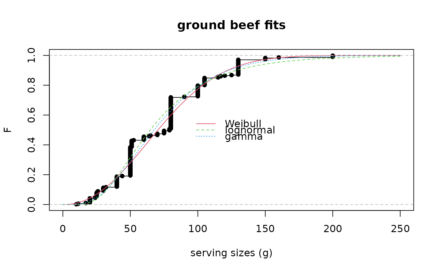
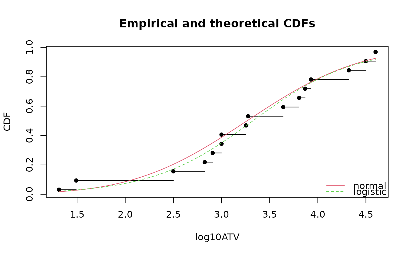
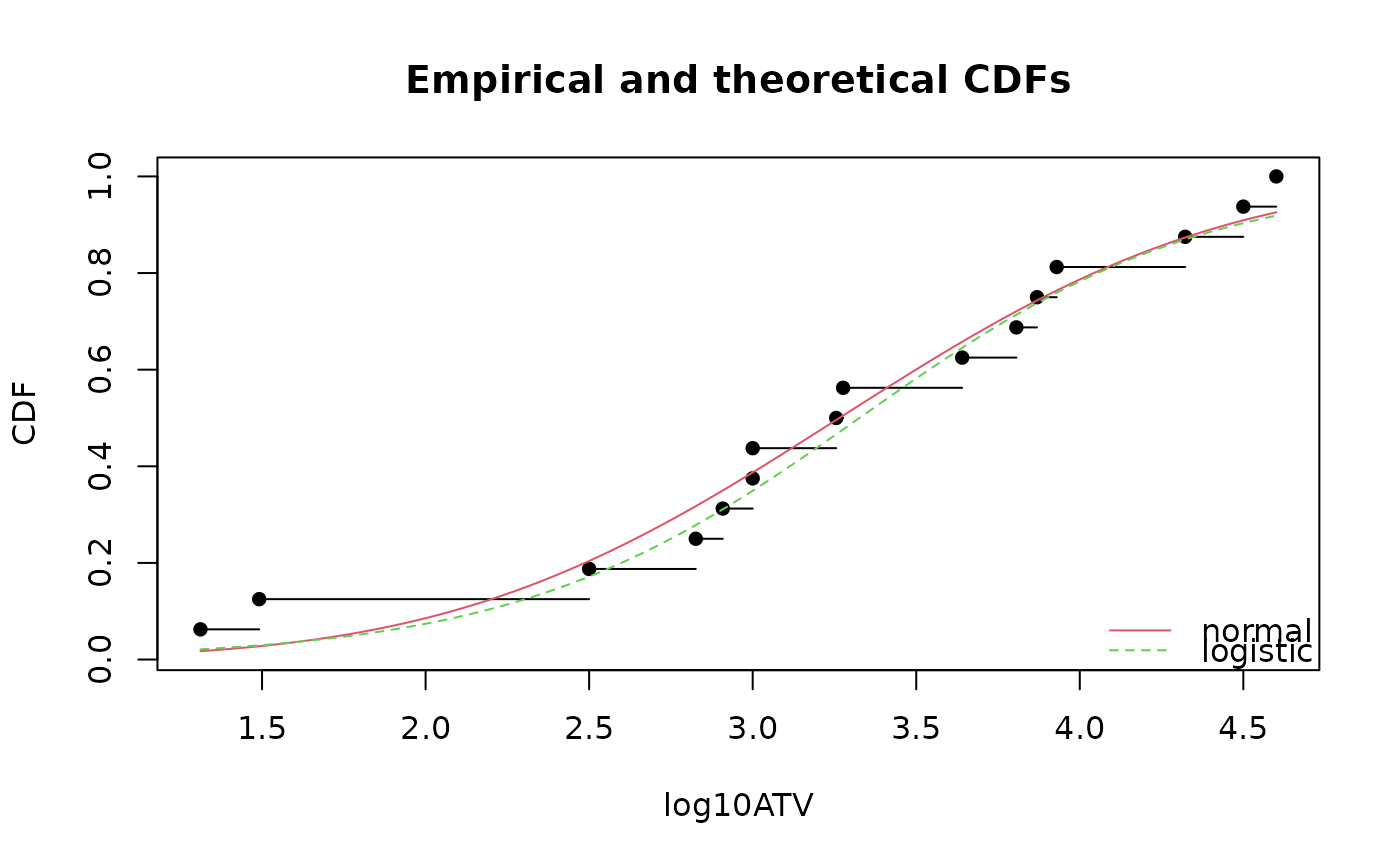
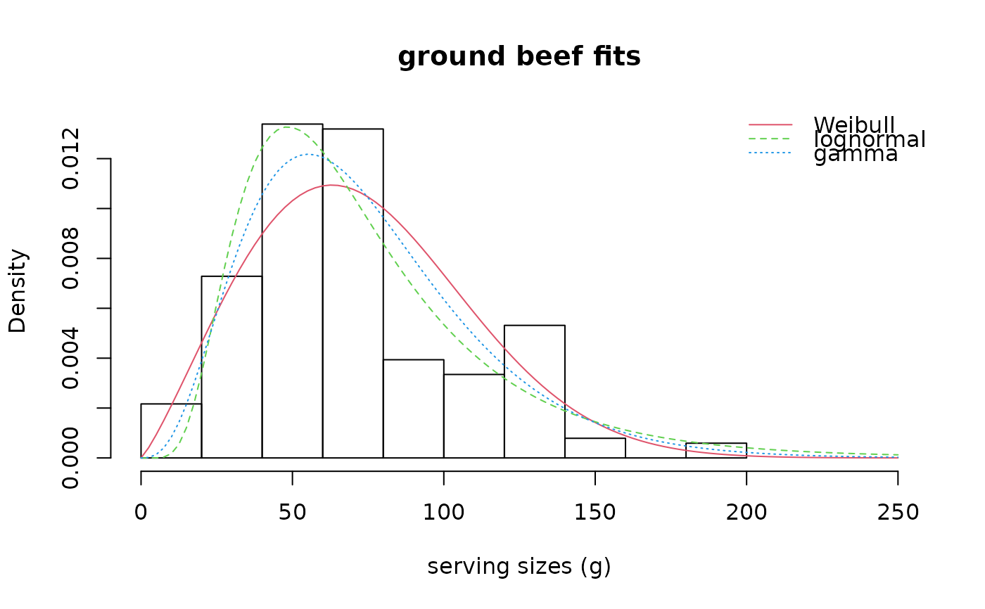
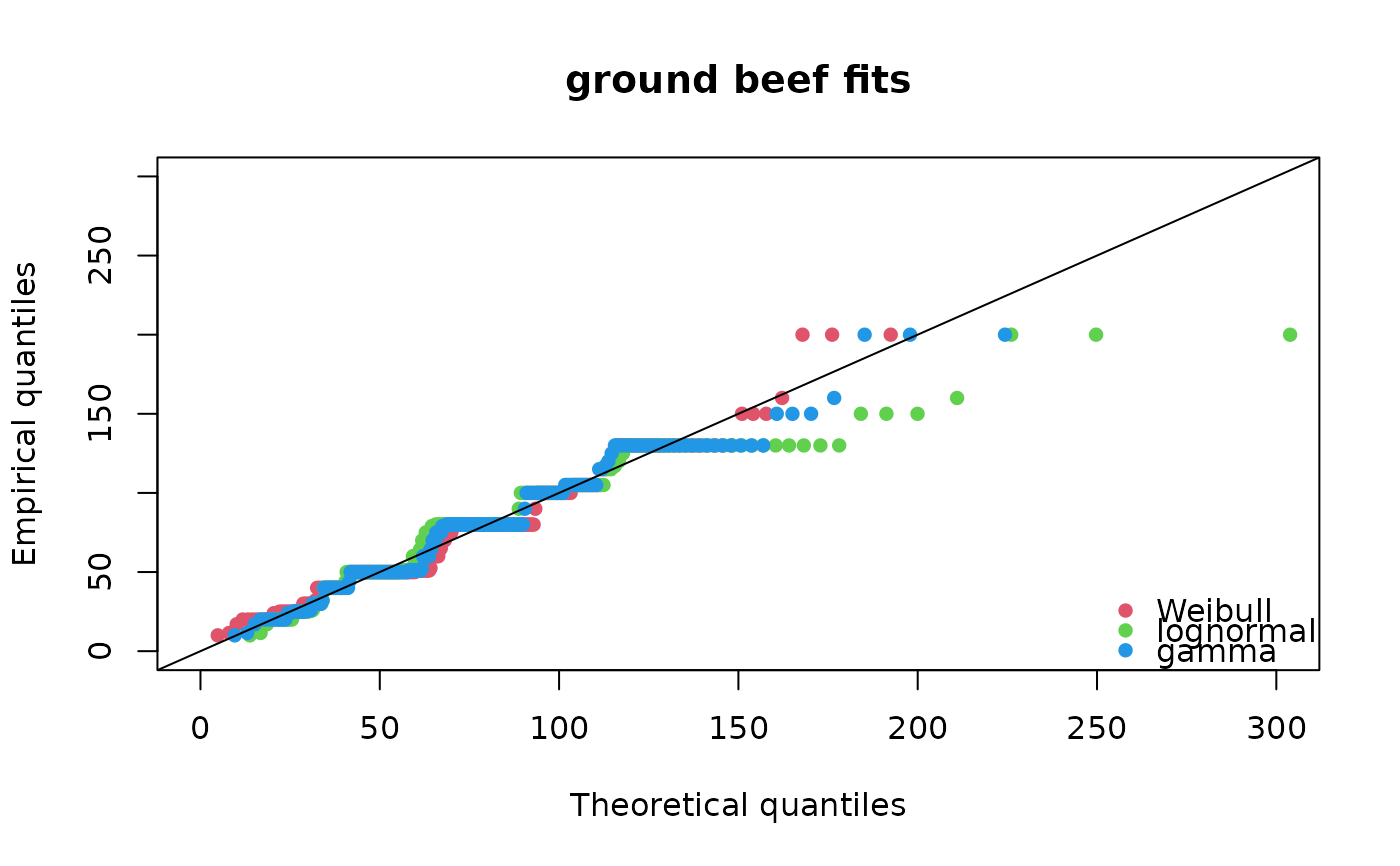
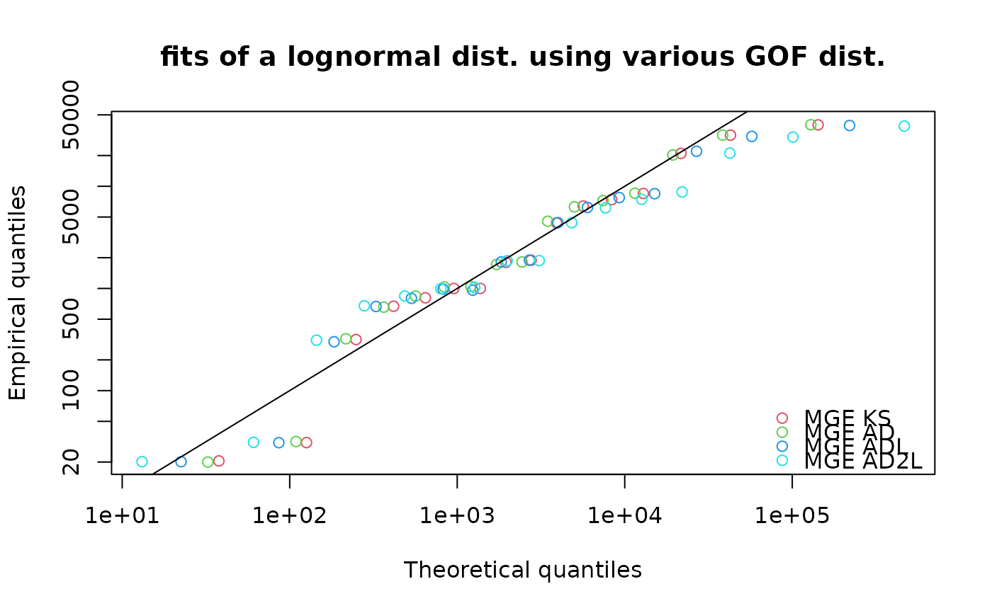
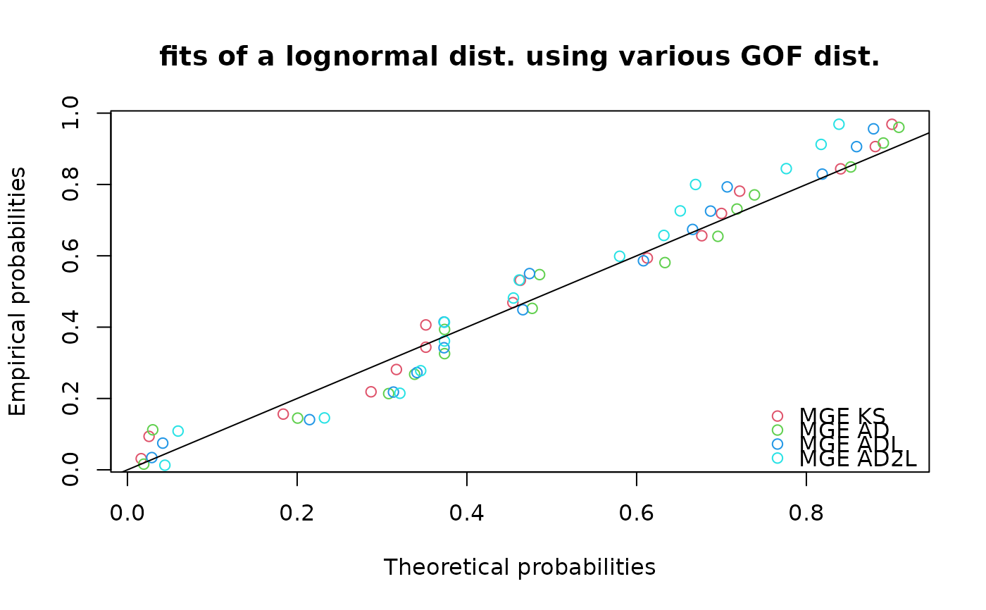
cdfcomp plots the empirical cumulative distribution against fitted distribution functions, denscomp plots the histogram against fitted density functions, qqcomp plots theoretical quantiles against empirical ones, ppcomp plots theoretical probabilities against empirical ones. Only cdfcomp is able to plot fits of a discrete distribution.

Usage

cdfcomp(ft, xlim, ylim, xlogscale = FALSE, ylogscale = FALSE, main, xlab, ylab, 
    datapch, datacol, fitlty, fitcol, fitlwd, addlegend = TRUE, legendtext, 
    xlegend = "bottomright", ylegend = NULL, horizontals = TRUE, verticals = FALSE, 
    do.points = TRUE, use.ppoints = TRUE, a.ppoints = 0.5, name.points = NULL,
    lines01 = FALSE, discrete, add = FALSE, plotstyle = "graphics", 
    fitnbpts = 101, ...)
    
denscomp(ft, xlim, ylim, probability = TRUE, main, xlab, ylab, datacol, fitlty, 
    fitcol, fitlwd, addlegend = TRUE, legendtext, xlegend = "topright", ylegend = NULL, 
    demp = FALSE, dempcol = "black", plotstyle = "graphics", 
    discrete, fitnbpts = 101, fittype="l", ...)

qqcomp(ft, xlim, ylim, xlogscale = FALSE, ylogscale = FALSE, main, xlab, ylab, 
    fitpch, fitcol, fitlwd, addlegend = TRUE, legendtext, xlegend = "bottomright", 
    ylegend = NULL, use.ppoints = TRUE, a.ppoints = 0.5, line01 = TRUE, 
    line01col = "black", line01lty = 1, ynoise = TRUE, plotstyle = "graphics", ...)
    
ppcomp(ft, xlim, ylim, xlogscale = FALSE, ylogscale = FALSE, main, xlab, ylab, 
    fitpch, fitcol, fitlwd, addlegend = TRUE, legendtext, xlegend = "bottomright", 
    ylegend = NULL, use.ppoints = TRUE, a.ppoints = 0.5, line01 = TRUE, 
    line01col = "black", line01lty = 1, ynoise = TRUE, plotstyle = "graphics", ...)

Arguments

ft: One "fitdist" object or a list of objects of class "fitdist".
xlim: The \(x\)-limits of the plot.
ylim: The \(y\)-limits of the plot.
xlogscale: If TRUE, uses a logarithmic scale for the \(x\)-axis.
ylogscale: If TRUE, uses a logarithmic scale for the \(y\)-axis.
main: A main title for the plot. See also title.
xlab: A label for the \(x\)-axis, defaults to a description of x.
ylab: A label for the \(y\)-axis, defaults to a description of y.
datapch: An integer specifying a symbol to be used in plotting data points. See also par.
datacol: A specification of the color to be used in plotting data points. See also par.
fitcol: A (vector of) color(s) to plot fitted distributions. If there are fewer colors than fits they are recycled in the standard fashion. See also par.
fitlty: A (vector of) line type(s) to plot fitted distributions/densities. If there are fewer values than fits they are recycled in the standard fashion. See also par.
fitlwd: A (vector of) line size(s) to plot fitted distributions/densities. If there are fewer values than fits they are recycled in the standard fashion. See also par.
fitpch: A (vector of) line type(s) to plot fitted quantiles/probabilities. If there are fewer values than fits they are recycled in the standard fashion. See also par.
fittype: The type of plot for fitted probabilities in the case of discrete distributions: possible types are "p" for points, "l" for lines and "o" for both overplotted (as in plot.default). fittype is not used for non-discrete distributions.
fitnbpts: A numeric for the number of points to compute fitted probabilities or cumulative probabilities. Default to 101.
addlegend: If TRUE, a legend is added to the plot.
legendtext: A character or expression vector of length \(\ge 1\) to appear in the legend. See also legend.
xlegend, ylegend: The \(x\) and \(y\) coordinates to be used to position the legend. They can be specified by keyword. If plotstyle = "graphics", see xy.coords and legend. If plotstyle = "ggplot", the xlegend keyword must be one of top, bottom, left, or right. See also guide_legend in ggplot2
horizontals: If TRUE, draws horizontal lines for the step empirical cumulative distribution function (ecdf). See also plot.stepfun.
verticals: If TRUE, draws vertical lines for the empirical cumulative distribution function (ecdf). Only taken into account if horizontals=TRUE.
do.points: If TRUE (by default), draws points at the x-locations. For large dataset (n > 1e4), do.points is ignored and no point is drawn.
use.ppoints: If TRUE, probability points of the empirical distribution are defined using function ppoints as (1:n - a.ppoints)/(n - 2a.ppoints + 1). If FALSE, probability points are simply defined as (1:n)/n. This argument is ignored for discrete data.
a.ppoints: If use.ppoints=TRUE, this is passed to the ppoints function.
name.points: Label vector for points if they are drawn i.e. if do.points = TRUE (only for non censored data).
lines01: A logical to plot two horizontal lines at h=0 and h=1 for cdfcomp.
line01: A logical to plot an horizontal line \(y=x\) for qqcomp and ppcomp.
line01col, line01lty: Color and line type for line01. See also par.
demp: A logical to add the empirical density on the plot, using the density function.
dempcol: A color for the empirical density in case it is added on the plot (demp=TRUE).
ynoise: A logical to add a small noise when plotting empirical quantiles/probabilities for qqcomp and ppcomp.
probability: A logical to use the probability scale for denscomp. See also hist.
discrete: If TRUE, the distributions are considered discrete. When missing, discrete is set to TRUE if at least one object of the list ft is discrete.
add: If TRUE, adds to an already existing plot. If FALSE, starts a new plot. This parameter is not available when plotstyle = "ggplot".
plotstyle: "graphics" or "ggplot". If "graphics", the display is built with graphics functions. If "ggplot", a graphic object output is created with ggplot2 functions (the ggplot2 package must be installed).
...: Further graphical arguments passed to graphical functions used in cdfcomp, denscomp, ppcomp and qqcomp when plotstyle = "graphics". When plotstyle = "ggplot", these arguments are only used by the histogram plot (hist) in the denscomp function. When plotstyle = "ggplot", the graphical output can be customized with relevant ggplot2 functions after you store your output.

Details

cdfcomp provides a plot of the empirical distribution and each fitted distribution in cdf, by default using the Hazen's rule for the empirical distribution, with probability points defined as (1:n - 0.5)/n. If discrete is TRUE, probability points are always defined as (1:n)/n. For large dataset (n > 1e4), no point is drawn but the line for ecdf is drawn instead. Note that when horizontals, verticals and do.points are FALSE, no empirical point is drawn, only the fitted cdf is shown.

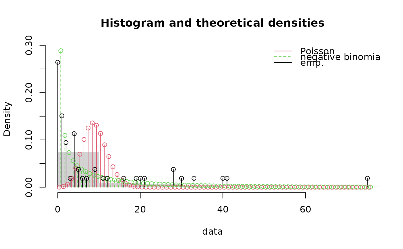
denscomp provides a density plot of each fitted distribution with the histogram of the data for conyinuous data. When discrete=TRUE, distributions are considered as discrete, no histogram is plotted but demp is forced to TRUE and fitted and empirical probabilities are plotted either with vertical lines fittype="l", with single points fittype="p" or both lines and points fittype="o".

ppcomp provides a plot of the probabilities of each fitted distribution (\(x\)-axis) against the empirical probabilities (\(y\)-axis) by default defined as (1:n - 0.5)/n (data are assumed continuous). For large dataset (n > 1e4), lines are drawn instead of pointss and customized with the fitpch parameter.

qqcomp provides a plot of the quantiles of each theoretical distribution (\(x\)-axis) against the empirical quantiles of the data (\(y\)-axis), by default defining probability points as (1:n - 0.5)/n for theoretical quantile calculation (data are assumed continuous). For large dataset (n > 1e4), lines are drawn instead of points and customized with the fitpch parameter.

By default a legend is added to these plots. Many graphical arguments are optional, dedicated to personalize the plots, and fixed to default values if omitted.

Value

*comp returns a list of drawn points and/or lines when plotstyle == "graphics" or an object of class "ggplot" when plotstyle == "ggplot".

References

Delignette-Muller ML and Dutang C (2015), fitdistrplus: An R Package for Fitting Distributions. Journal of Statistical Software, 64(4), 1-34, doi:10.18637/jss.v064.i04 .

Author

Christophe Dutang, Marie-Laure Delignette-Muller and Aurelie Siberchicot.

Examples

# (1) Plot various distributions fitted to serving size data
#
data(groundbeef)
serving <- groundbeef$serving
fitW <- fitdist(serving, "weibull")
fitln <- fitdist(serving, "lnorm")
fitg <- fitdist(serving, "gamma")

cdfcomp(list(fitW, fitln, fitg), horizontals = FALSE)

cdfcomp(list(fitW, fitln, fitg), horizontals = TRUE)

cdfcomp(list(fitW, fitln, fitg), horizontals = TRUE, verticals = TRUE, datacol = "purple")

cdfcomp(list(fitW, fitln, fitg), legendtext = c("Weibull", "lognormal", "gamma"),
  main = "ground beef fits", xlab = "serving sizes (g)",
  ylab = "F", xlim = c(0, 250), xlegend = "center", lines01 = TRUE)

denscomp(list(fitW, fitln, fitg), legendtext = c("Weibull", "lognormal", "gamma"),
  main = "ground beef fits", xlab = "serving sizes (g)", xlim = c(0, 250), xlegend = "topright")

ppcomp(list(fitW, fitln, fitg), legendtext = c("Weibull", "lognormal", "gamma"),
  main = "ground beef fits", xlegend = "bottomright", line01 = TRUE)

qqcomp(list(fitW, fitln, fitg), legendtext = c("Weibull", "lognormal", "gamma"),
  main = "ground beef fits", xlegend = "bottomright", line01 = TRUE,
  xlim = c(0, 300), ylim = c(0, 300), fitpch = 16)



# (2) Plot lognormal distributions fitted by 
# maximum goodness-of-fit estimation
# using various distances (data plotted in log scale)
#
data(endosulfan)
ATV <- subset(endosulfan, group == "NonArthroInvert")$ATV
taxaATV <- subset(endosulfan, group == "NonArthroInvert")$taxa
flnMGEKS <- fitdist(ATV, "lnorm", method = "mge", gof = "KS")
flnMGEAD <- fitdist(ATV, "lnorm", method = "mge", gof = "AD")
flnMGEADL <- fitdist(ATV, "lnorm", method = "mge", gof = "ADL")
flnMGEAD2L <- fitdist(ATV, "lnorm", method = "mge", gof = "AD2L")

cdfcomp(list(flnMGEKS, flnMGEAD, flnMGEADL, flnMGEAD2L),
  xlogscale = TRUE, main = "fits of a lognormal dist. using various GOF dist.",
  legendtext = c("MGE KS", "MGE AD", "MGE ADL", "MGE AD2L"),
  verticals = TRUE, xlim = c(1, 100000), name.points=taxaATV)

qqcomp(list(flnMGEKS, flnMGEAD, flnMGEADL, flnMGEAD2L),
  main = "fits of a lognormal dist. using various GOF dist.",
  legendtext = c("MGE KS", "MGE AD", "MGE ADL", "MGE AD2L"),
  xlogscale = TRUE, ylogscale = TRUE)

ppcomp(list(flnMGEKS, flnMGEAD, flnMGEADL, flnMGEAD2L),
  main = "fits of a lognormal dist. using various GOF dist.",
  legendtext = c("MGE KS", "MGE AD", "MGE ADL", "MGE AD2L"))



# (3) Plot normal and logistic distributions fitted by 
# maximum likelihood estimation
# using various plotting positions in cdf plots
#
data(endosulfan)
log10ATV <-log10(subset(endosulfan, group == "NonArthroInvert")$ATV)
fln <- fitdist(log10ATV, "norm")
fll <- fitdist(log10ATV, "logis")

# default plot using Hazen plotting position: (1:n - 0.5)/n
cdfcomp(list(fln, fll), legendtext = c("normal", "logistic"), xlab = "log10ATV")


# plot using mean plotting position (named also Gumbel plotting position)
# (1:n)/(n + 1)
cdfcomp(list(fln, fll),legendtext = c("normal", "logistic"), xlab = "log10ATV",
  use.ppoints = TRUE, a.ppoints = 0)

    
# plot using basic plotting position: (1:n)/n
cdfcomp(list(fln, fll),legendtext = c("normal", "logistic"), xlab = "log10ATV",
  use.ppoints = FALSE)



# (4) Comparison of fits of two distributions fitted to discrete data
#
data(toxocara)
number <- toxocara$number
fitp <- fitdist(number, "pois")
fitnb <- fitdist(number, "nbinom")
cdfcomp(list(fitp, fitnb), legendtext = c("Poisson", "negative binomial"))

denscomp(list(fitp, fitnb),demp = TRUE, legendtext = c("Poisson", "negative binomial"))

denscomp(list(fitp, fitnb),demp = TRUE, fittype = "l", dempcol = "black",
  legendtext = c("Poisson", "negative binomial"))
denscomp(list(fitp, fitnb),demp = TRUE, fittype = "p", dempcol = "black",
  legendtext = c("Poisson", "negative binomial"))

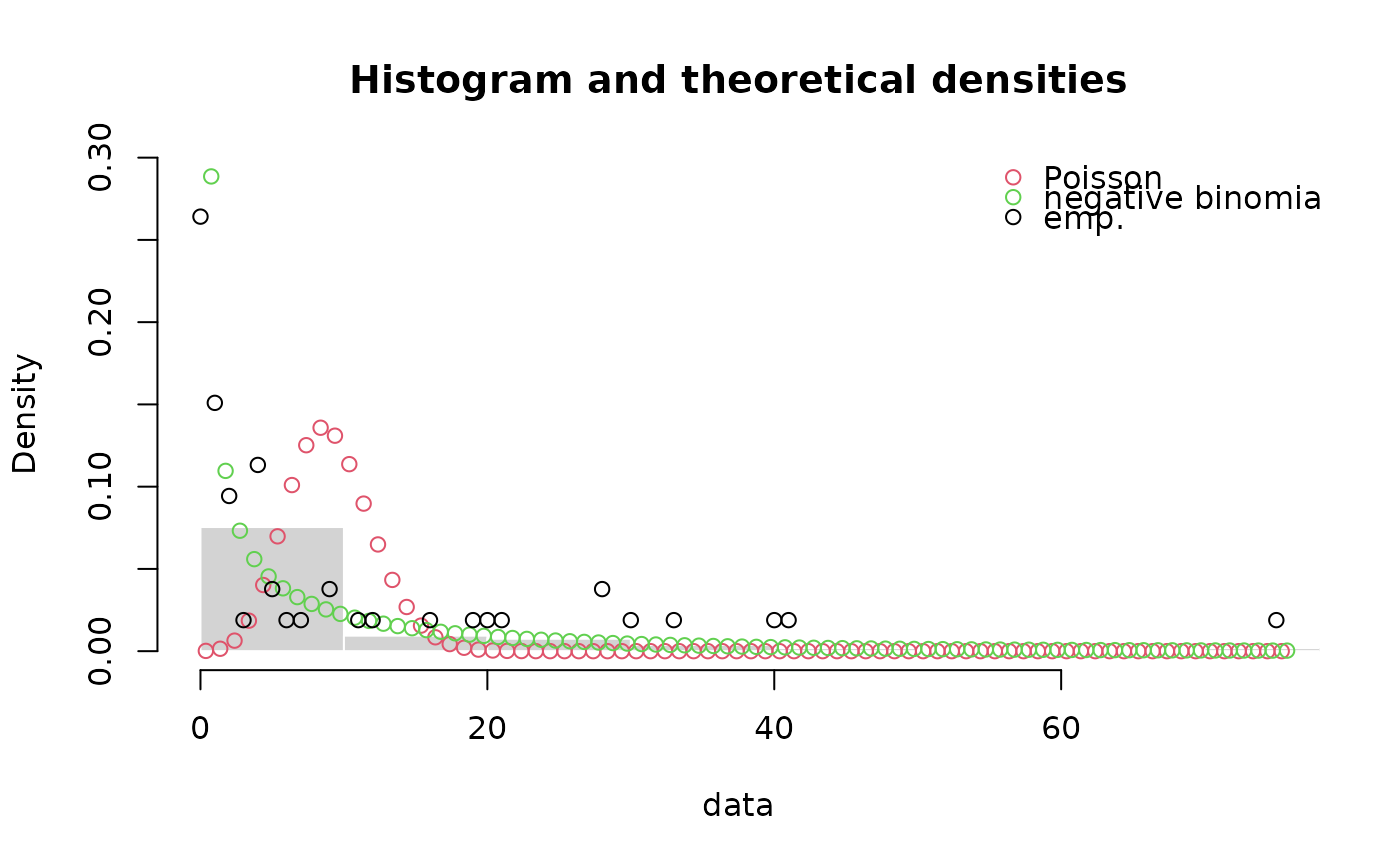denscomp(list(fitp, fitnb),demp = TRUE, fittype = "o", dempcol = "black",
  legendtext = c("Poisson", "negative binomial"))



# (5) Customizing of graphical output and use of ggplot2
#
data(groundbeef)
serving <- groundbeef$serving
fitW <- fitdist(serving, "weibull")
fitln <- fitdist(serving, "lnorm")
fitg <- fitdist(serving, "gamma")
if (requireNamespace ("ggplot2", quietly = TRUE)) {
  denscomp(list(fitW, fitln, fitg), plotstyle = "ggplot")
  cdfcomp(list(fitW, fitln, fitg), plotstyle = "ggplot")
  qqcomp(list(fitW, fitln, fitg), plotstyle = "ggplot")
  ppcomp(list(fitW, fitln, fitg), plotstyle = "ggplot")
}


# customizing graphical output with graphics
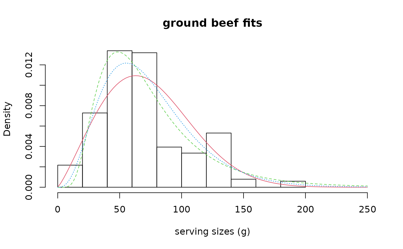
denscomp(list(fitW, fitln, fitg), legendtext = c("Weibull", "lognormal", "gamma"),
  main = "ground beef fits", xlab = "serving sizes (g)", xlim = c(0, 250),
  xlegend = "topright", addlegend = FALSE)


# customizing graphical output with ggplot2
if (requireNamespace ("ggplot2", quietly = TRUE)) {
  dcomp <- denscomp(list(fitW, fitln, fitg), legendtext = c("Weibull", "lognormal", "gamma"),
    xlab = "serving sizes (g)", xlim = c(0, 250),
    xlegend = "topright", plotstyle = "ggplot", breaks = 20, addlegend = FALSE)
  dcomp + ggplot2::theme_minimal() + ggplot2::ggtitle("Ground beef fits")
}