Empirical cumulative distribution function with pointwise confidence intervals on probabilities or on quantiles

cdfband plots the empirical cumulative distribution function with the bootstraped pointwise confidence intervals on probabilities of on quantiles.

Usage

CIcdfplot(b, CI.output, CI.type = "two.sided", CI.level = 0.95, CI.col = "red", 
  CI.lty = 2, CI.fill = NULL, CI.only = FALSE, xlim, ylim, xlogscale = FALSE, 
  ylogscale = FALSE, main, xlab, ylab, datapch, datacol, fitlty, fitcol, fitlwd, 
  horizontals = TRUE, verticals = FALSE, do.points = TRUE, use.ppoints = TRUE, 
  a.ppoints = 0.5, name.points = NULL, lines01 = FALSE, plotstyle = "graphics", ...)

Arguments

b: One "bootdist" object.
CI.output: The quantity on which (bootstraped) bootstraped confidence intervals are computed: either "probability" or "quantile").
CI.type: Type of confidence intervals : either "two.sided" or one-sided intervals ("less" or "greater").
CI.level: The confidence level.
CI.col: the color of the confidence intervals.
CI.lty: the line type of the confidence intervals.
CI.fill: a color to fill the confidence area. Default is NULL corresponding to no filling.
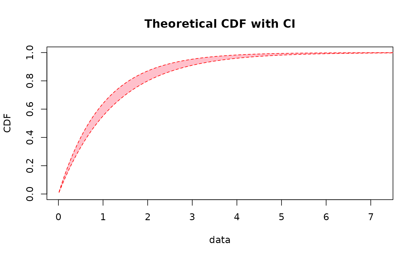
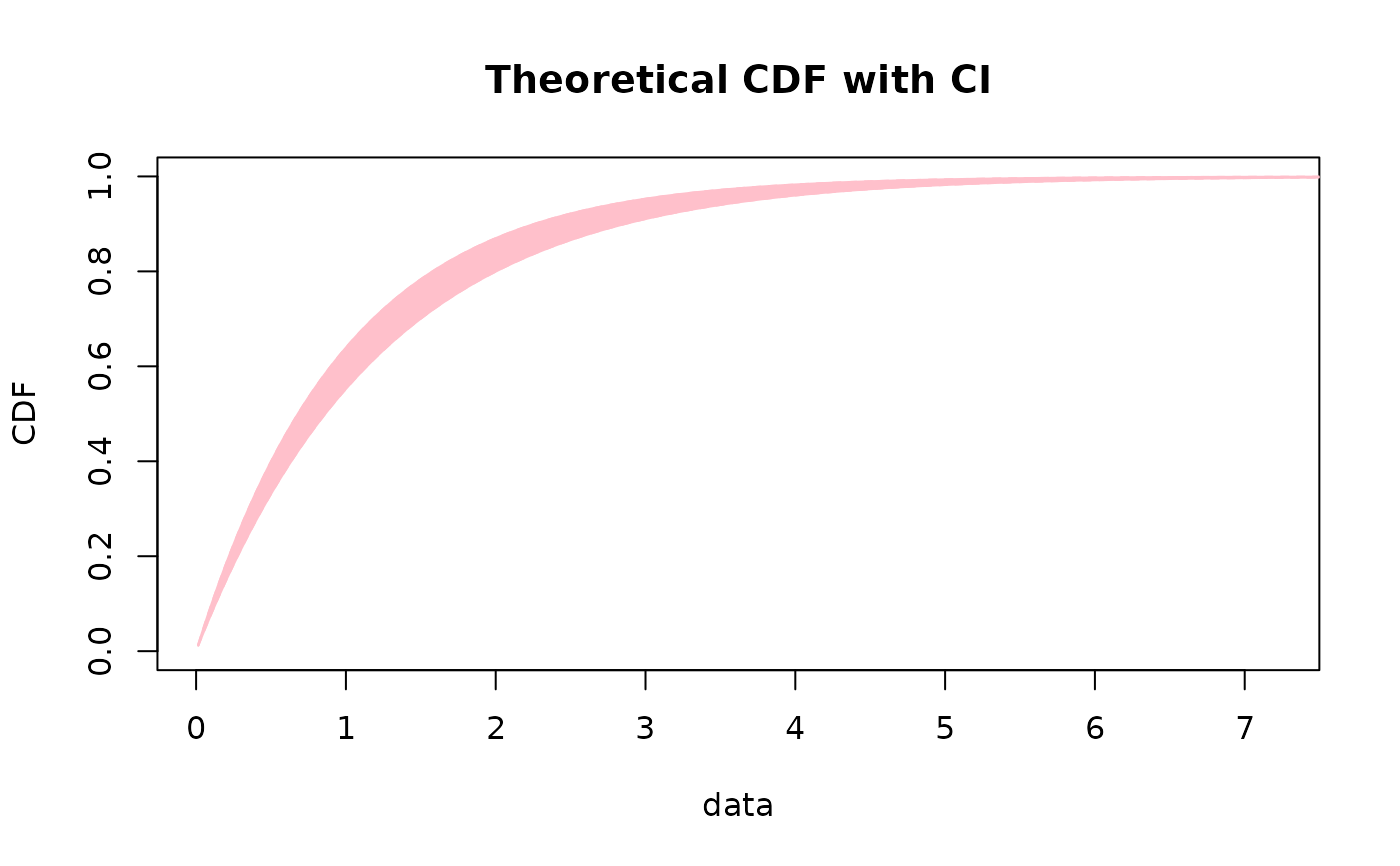
CI.only: A logical whether to plot empirical and fitted distribution functions or only the confidence intervals. Default to FALSE.
xlim: The \(x\)-limits of the plot.
ylim: The \(y\)-limits of the plot.
xlogscale: If TRUE, uses a logarithmic scale for the \(x\)-axis.
ylogscale: If TRUE, uses a logarithmic scale for the \(y\)-axis.
main: A main title for the plot, see also title.
xlab: A label for the \(x\)-axis, defaults to a description of x.
ylab: A label for the \(y\)-axis, defaults to a description of y.
datapch: An integer specifying a symbol to be used in plotting data points, see also points (only for non censored data).
datacol: A specification of the color to be used in plotting data points.
fitcol: A (vector of) color(s) to plot fitted distributions. If there are fewer colors than fits they are recycled in the standard fashion.
fitlty: A (vector of) line type(s) to plot fitted distributions/densities. If there are fewer values than fits they are recycled in the standard fashion. See also par.
fitlwd: A (vector of) line size(s) to plot fitted distributions/densities. If there are fewer values than fits they are recycled in the standard fashion. See also par.
horizontals: If TRUE, draws horizontal lines for the step empirical cdf function (only for non censored data). See also plot.stepfun.
verticals: If TRUE, draws also vertical lines for the empirical cdf function. Only taken into account if horizontals=TRUE (only for non censored data).
do.points: logical; if TRUE, also draw points at the x-locations. Default is TRUE (only for non censored data).
use.ppoints: If TRUE, probability points of the empirical distribution are defined using function ppoints as (1:n - a.ppoints)/(n - 2a.ppoints + 1) (only for non censored data). If FALSE, probability points are simply defined as (1:n)/n. This argument is ignored for discrete data.
a.ppoints: If use.ppoints=TRUE, this is passed to function ppoints (only for non censored data).
name.points: Label vector for points if they are drawn i.e. if do.points = TRUE (only for non censored data).
lines01: A logical to plot two horizontal lines at h=0 and h=1 for cdfcomp.
plotstyle: "graphics" or "ggplot". If "graphics", the display is built with graphics functions. If "ggplot", a graphic object output is created with ggplot2 functions (the ggplot2 package must be installed).
...: Further graphical arguments passed to matlines or polygon, respectively when CI.fill=FALSE and CI.fill=TRUE.

Details

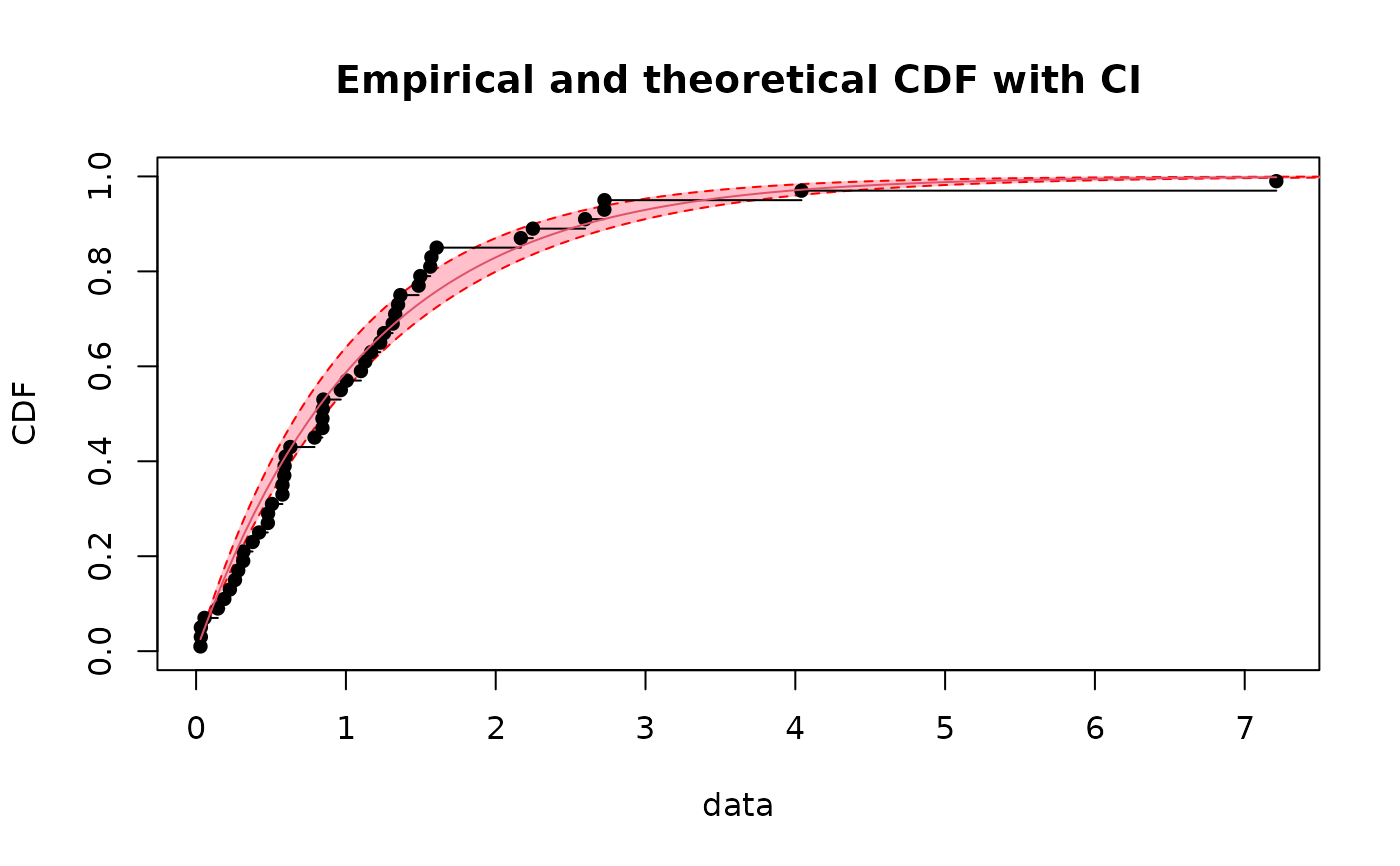
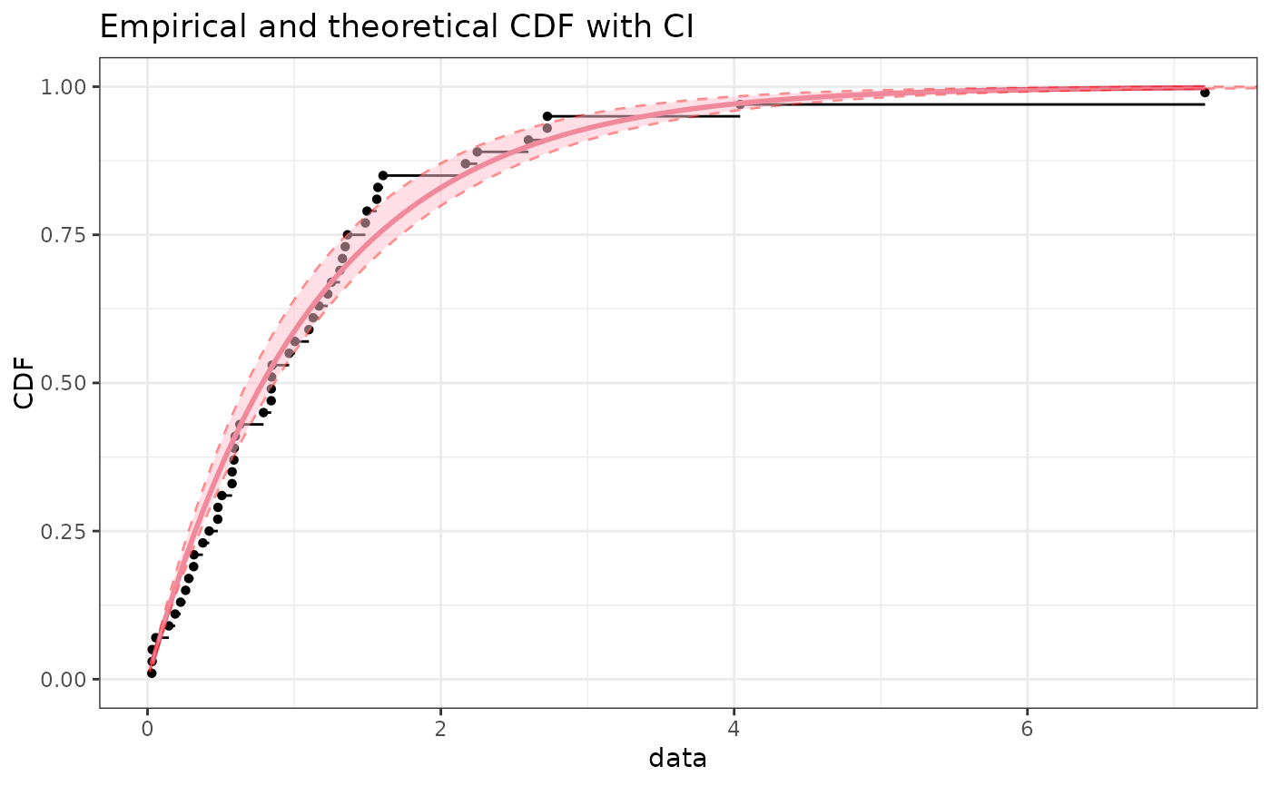
CIcdfplot provides a plot of the empirical distribution using cdfcomp or cdfcompcens, with bootstraped pointwise confidence intervals on probabilities (y values) or on quantiles (x values). Each interval is computed by evaluating the quantity of interest (probability associated to an x value or quantile associated to an y value) using all the bootstraped values of parameters to get a bootstraped sample of the quantity of interest and then by calculating percentiles on this sample to get a confidence interval (classically 2.5 and 97.5 percentiles for a 95 percent confidence level). If CI.fill != NULL, then the whole confidence area is filled by the color CI.fill thanks to the function polygon, otherwise only borders are drawn thanks to the function matline. Further graphical arguments can be passed to these functions using the three dots arguments ....

References

Delignette-Muller ML and Dutang C (2015), fitdistrplus: An R Package for Fitting Distributions. Journal of Statistical Software, 64(4), 1-34, doi:10.18637/jss.v064.i04 .

Author

Christophe Dutang and Marie-Laure Delignette-Muller.

Examples

# We choose a low number of bootstrap replicates in order to satisfy CRAN running times
# constraint.
# For practical applications, we recommend to use at least niter=501 or niter=1001.

if (requireNamespace ("ggplot2", quietly = TRUE)) {ggplotEx <- TRUE}

# (1) Fit of an exponential distribution
#

set.seed(123)
s1 <- rexp(50, 1)
f1 <- fitdist(s1, "exp")
b1 <- bootdist(f1, niter= 11) #voluntarily low to decrease computation time

# plot 95 percent bilateral confidence intervals on y values (probabilities)
CIcdfplot(b1, CI.level= 95/100, CI.output = "probability")

if (ggplotEx) CIcdfplot(b1, CI.level= 95/100, CI.output = "probability", plotstyle = "ggplot")


# \donttest{
# plot of the previous intervals as a band 
CIcdfplot(b1, CI.level= 95/100, CI.output = "probability", 
  CI.fill = "pink", CI.col = "red")

if (ggplotEx) CIcdfplot(b1, CI.level= 95/100, CI.output = "probability", 
  CI.fill = "pink", CI.col = "red", plotstyle = "ggplot")


# plot of the previous intervals as a band without empirical and fitted dist. functions
CIcdfplot(b1, CI.level= 95/100, CI.output = "probability", CI.only = TRUE,
  CI.fill = "pink", CI.col = "red")

if (ggplotEx) CIcdfplot(b1, CI.level= 95/100, CI.output = "probability", CI.only = TRUE,
  CI.fill = "pink", CI.col = "red", plotstyle = "ggplot")

  
# same plot without contours
CIcdfplot(b1, CI.level= 95/100, CI.output = "probability", CI.only = TRUE,
  CI.fill = "pink", CI.col = "pink")

if (ggplotEx) CIcdfplot(b1, CI.level= 95/100, CI.output = "probability", CI.only = TRUE,
  CI.fill = "pink", CI.col = "pink", plotstyle = "ggplot")


# plot 95 percent bilateral confidence intervals on x values (quantiles)
CIcdfplot(b1, CI.level= 95/100, CI.output = "quantile")

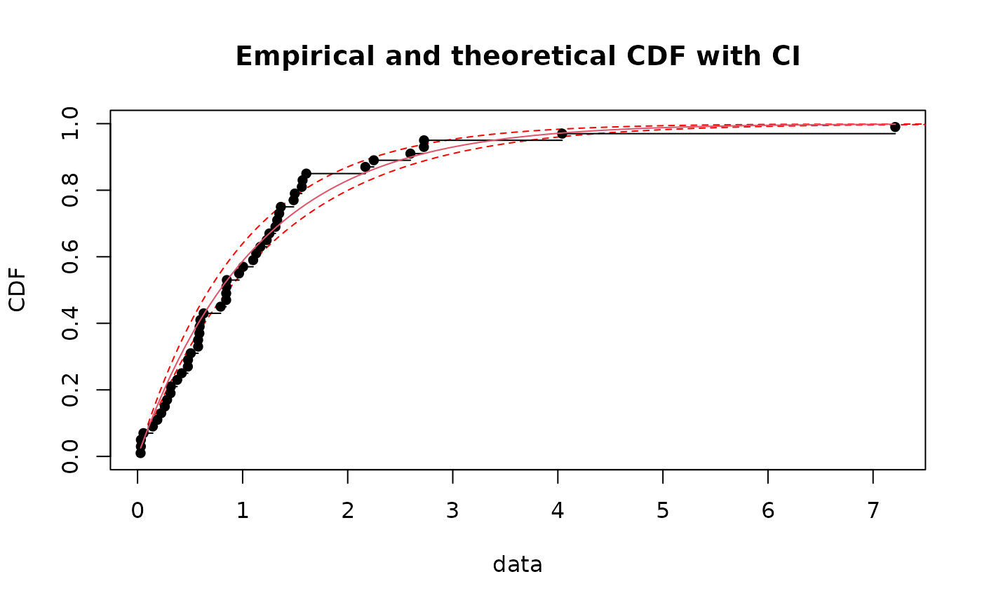if (ggplotEx) CIcdfplot(b1, CI.level= 95/100, CI.output = "quantile", plotstyle = "ggplot")



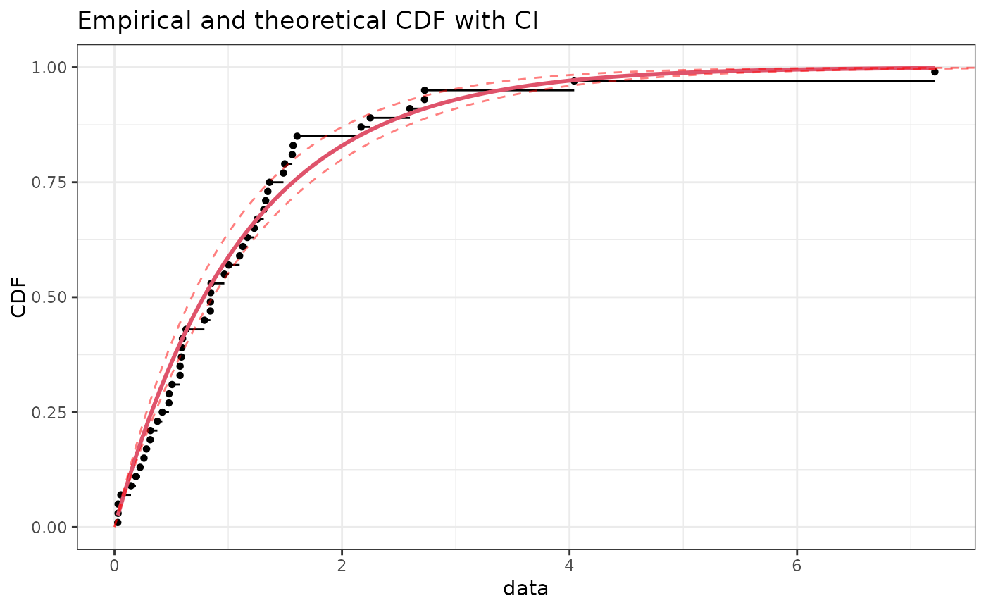# plot 95 percent unilateral confidence intervals on quantiles
CIcdfplot(b1, CI.level = 95/100, CI.output = "quant", CI.type = "less", 
  CI.fill = "grey80", CI.col = "black", CI.lty = 1)

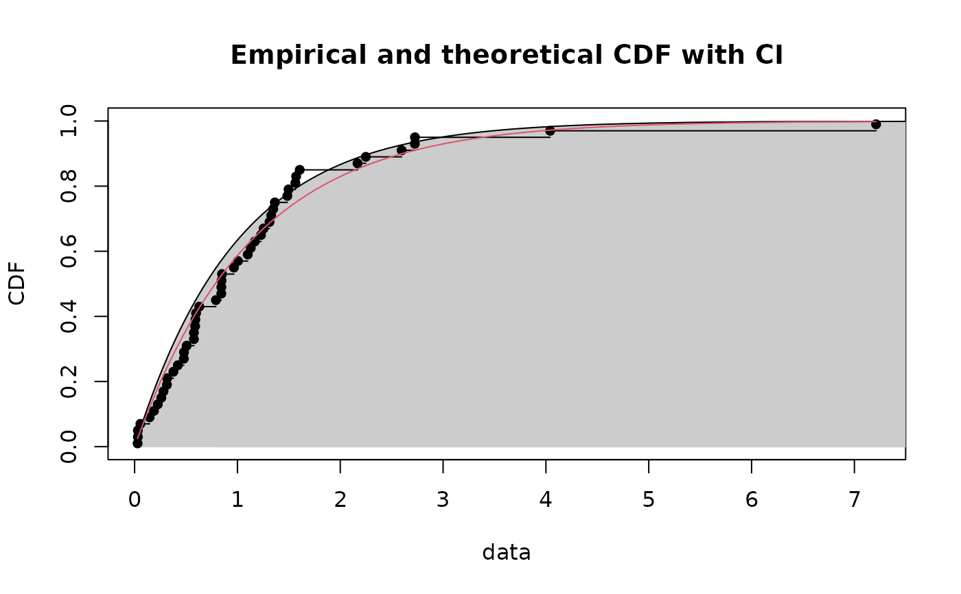if (ggplotEx) CIcdfplot(b1, CI.level = 95/100, CI.output = "quant", CI.type = "less", 
  CI.fill = "grey80", CI.col = "black", CI.lty = 1, plotstyle = "ggplot")

    
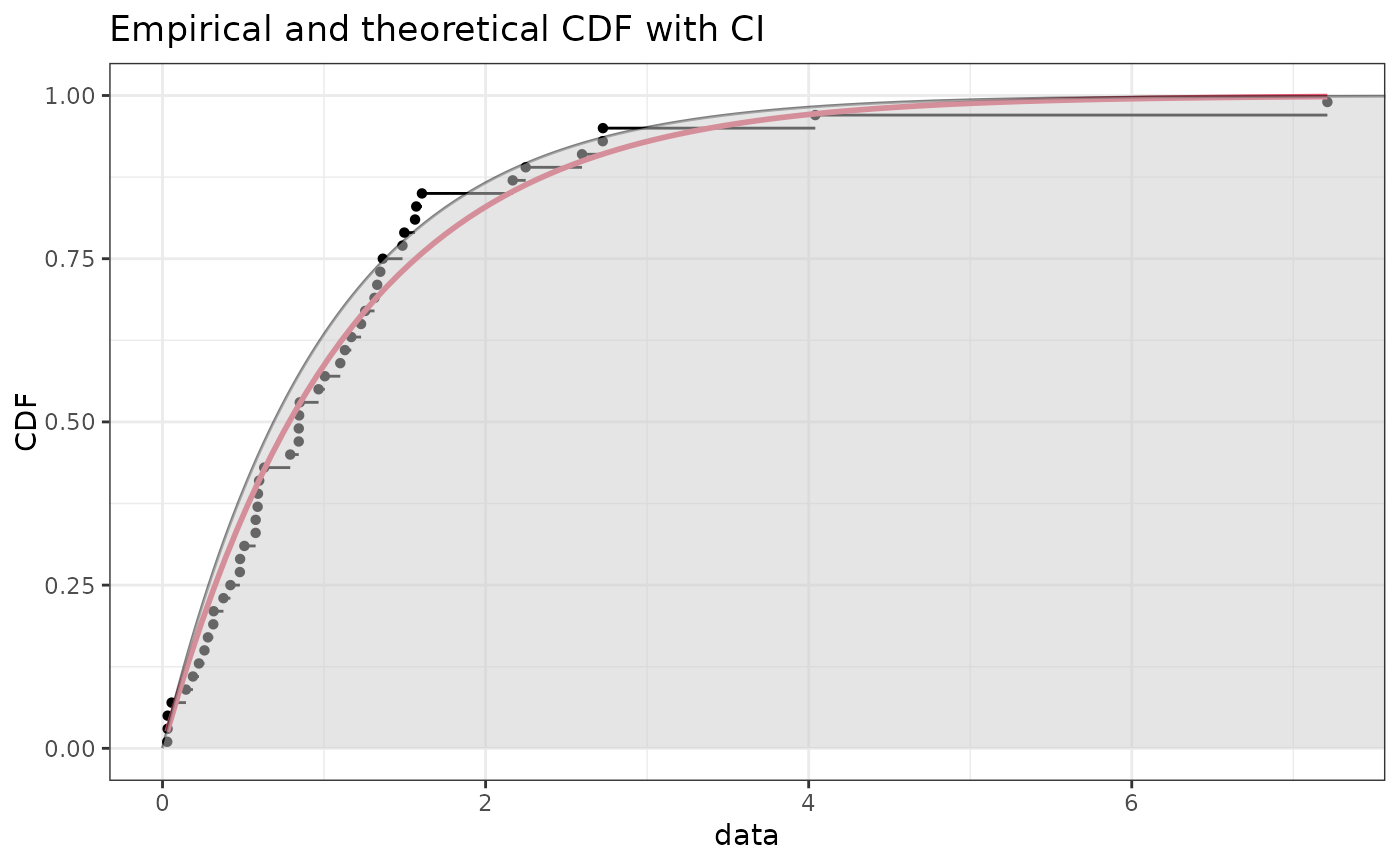CIcdfplot(b1, CI.level= 95/100, CI.output = "quant", CI.type = "greater",
  CI.fill = "grey80", CI.col = "black", CI.lty = 1)

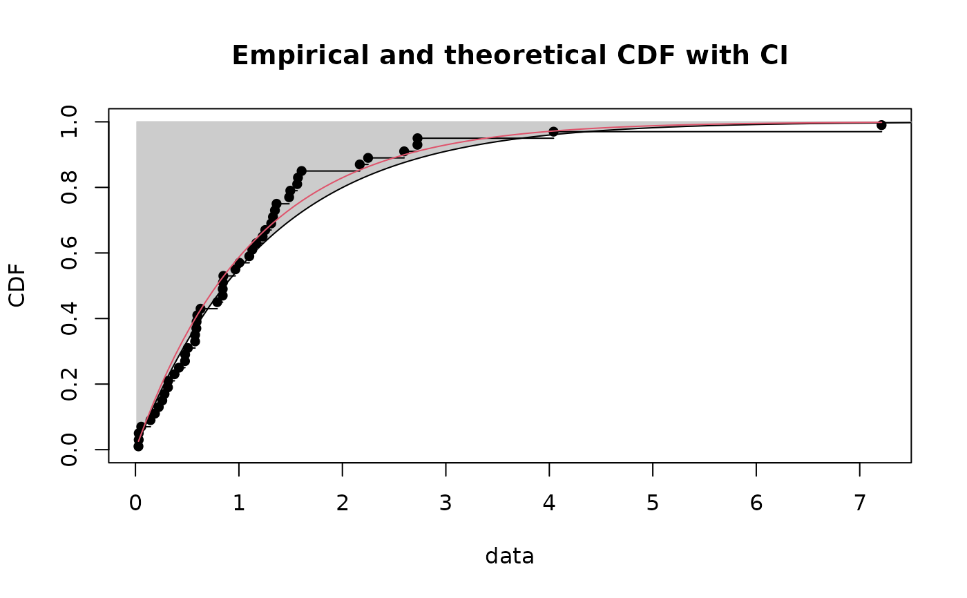if (ggplotEx) CIcdfplot(b1, CI.level= 95/100, CI.output = "quant", CI.type = "greater",
  CI.fill = "grey80", CI.col = "black", CI.lty = 1, plotstyle = "ggplot")


# (2) Fit of a normal distribution on acute toxicity log-transformed values of 
# endosulfan for nonarthropod invertebrates, using maximum likelihood estimation
# to estimate what is called a species sensitivity distribution 
# (SSD) in ecotoxicology, followed by estimation of the 5, 10 and 20 percent quantile  
# values of the fitted distribution, which are called the 5, 10, 20 percent hazardous 
# concentrations (HC5, HC10, HC20) in ecotoxicology, with their
# confidence intervals, from a small number of bootstrap 
# iterations to satisfy CRAN running times constraint and plot of the band
# representing pointwise confidence intervals on any quantiles (any HCx values)
# For practical applications, we recommend to use at least niter=501 or niter=1001.
#

data(endosulfan)
log10ATV <- log10(subset(endosulfan, group == "NonArthroInvert")$ATV)
namesATV <- subset(endosulfan, group == "NonArthroInvert")$taxa
fln <- fitdist(log10ATV, "norm")
bln <- bootdist(fln, bootmethod ="param", niter=101)
quantile(bln, probs = c(0.05, 0.1, 0.2))
#> (original) estimated quantiles for each specified probability (non-censored data)
#>            p=0.05    p=0.1  p=0.2
#> estimate 1.744227 2.080093 2.4868
#> Median of bootstrap estimates
#>            p=0.05    p=0.1    p=0.2
#> estimate 1.844443 2.190122 2.565053
#> 
#> two-sided 95 % CI of each quantile
#>          p=0.05    p=0.1    p=0.2
#> 2.5 %  1.334340 1.697255 2.099378
#> 97.5 % 2.531564 2.770455 3.053706
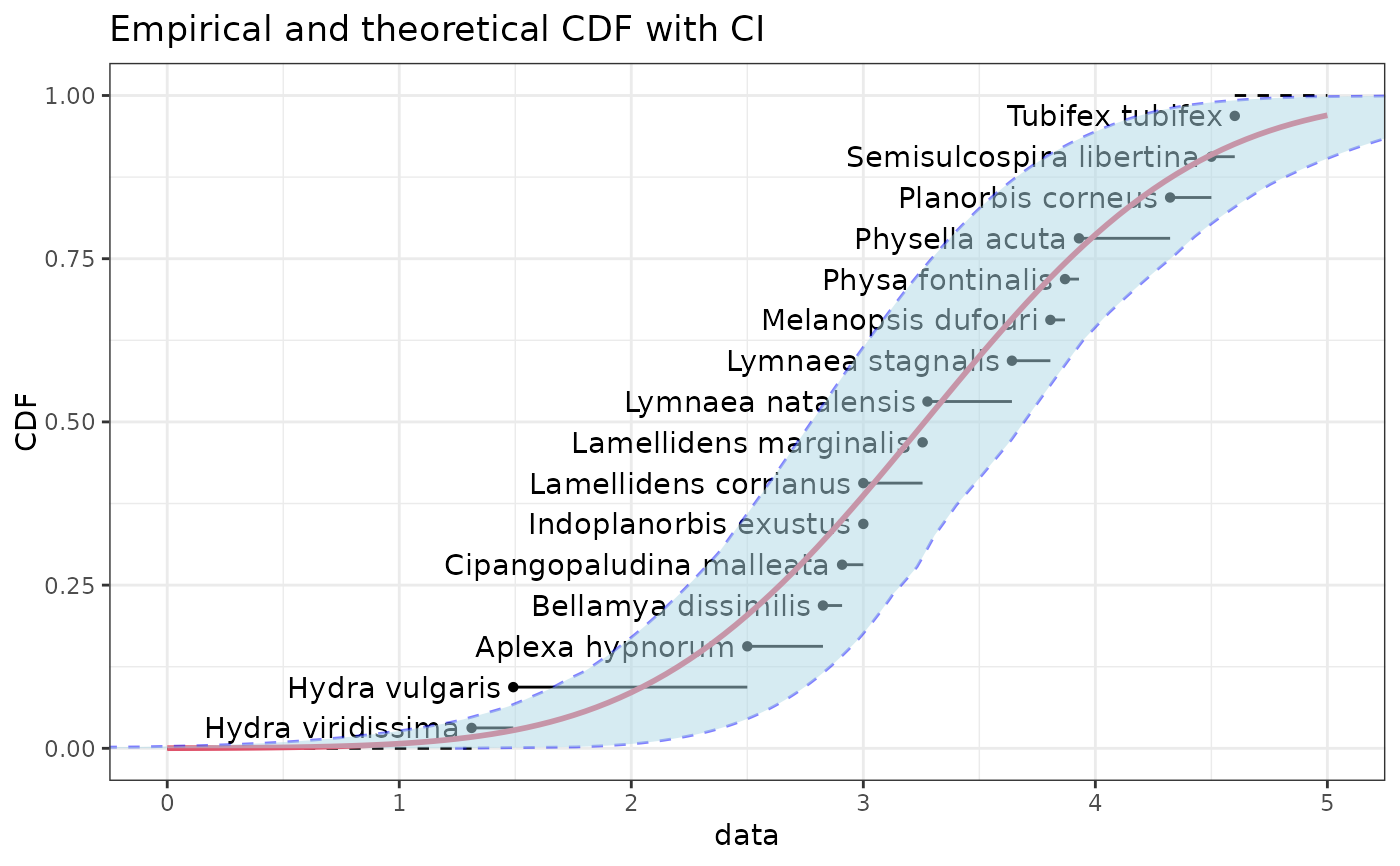
CIcdfplot(bln, CI.output = "quantile", CI.fill = "lightblue", CI.col = "blue",
          xlim = c(0,5), name.points=namesATV)

if (ggplotEx) CIcdfplot(bln, CI.output = "quantile", CI.fill = "lightblue", CI.col = "blue",
  xlim = c(0,5), name.points=namesATV, plotstyle = "ggplot")



# (3) Same type of example as example (2) from ecotoxicology
# with censored data
#
data(salinity)
log10LC50 <-log10(salinity)
fln <- fitdistcens(log10LC50,"norm")
bln <- bootdistcens(fln, niter=101)
(HC5ln <- quantile(bln,probs = 0.05))
#> (original) estimated quantiles for each specified probability (censored data)
#>           p=0.05
#> estimate 1.11584
#> Median of bootstrap estimates
#>            p=0.05
#> estimate 1.120901
#> 
#> two-sided 95 % CI of each quantile
#>          p=0.05
#> 2.5 %  1.045539
#> 97.5 % 1.191979
CIcdfplot(bln, CI.output = "quantile", CI.fill = "lightblue", CI.col = "blue",
    xlab = "log10(LC50)",xlim=c(0.5,2),lines01 = TRUE)

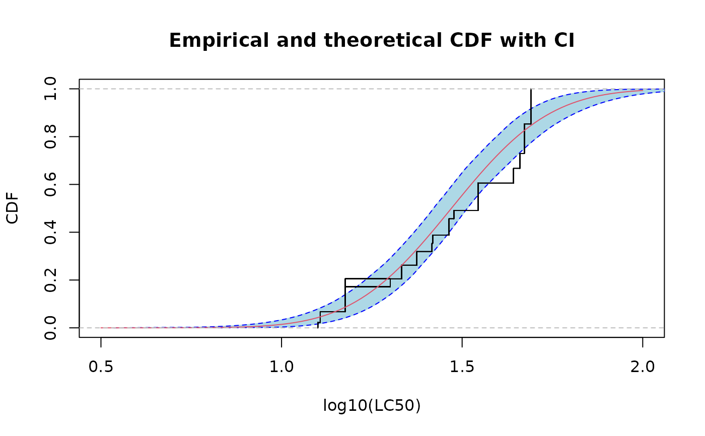if (ggplotEx) CIcdfplot(bln, CI.output = "quantile", CI.fill = "lightblue", CI.col = "blue",
                        xlab = "log10(LC50)",xlim=c(0.5,2),lines01 = TRUE, plotstyle = "ggplot")

# zoom around the HC5  
CIcdfplot(bln, CI.output = "quantile", CI.fill = "lightblue", CI.col = "blue",
          xlab = "log10(LC50)", lines01 = TRUE, xlim = c(0.8, 1.5), ylim = c(0, 0.1))
abline(h = 0.05, lty = 2) # line corresponding to a CDF of 5 percent


if (ggplotEx) CIcdfplot(bln, CI.output = "quantile", CI.fill = "lightblue", CI.col = "blue",
    xlab = "log10(LC50)", lines01 = TRUE, xlim = c(0.8, 1.5), ylim = c(0, 0.1), 
    plotstyle = "ggplot") +
  ggplot2::geom_hline(yintercept = 0.05, lty = 2) # line corresponding to a CDF of 5 percent

# }