Fitting of univariate distributions to censored data
fitdistcens.RdFits a univariate distribution to censored data by maximum likelihood.
Usage
fitdistcens(censdata, distr, start=NULL, fix.arg=NULL,
  keepdata = TRUE, keepdata.nb=100, calcvcov=TRUE, ...)

# S3 method for class 'fitdistcens'
print(x, ...)

# S3 method for class 'fitdistcens'
plot(x, ...)

# S3 method for class 'fitdistcens'
summary(object, ...)

# S3 method for class 'fitdistcens'
logLik(object, ...)

# S3 method for class 'fitdistcens'
AIC(object, ..., k = 2)

# S3 method for class 'fitdistcens'
BIC(object, ...)

# S3 method for class 'fitdistcens'
vcov(object, ...)

# S3 method for class 'fitdistcens'
coef(object, ...)
Arguments
- censdata
A dataframe of two columns respectively named
leftandright, describing each observed value as an interval. Theleftcolumn contains eitherNAfor left censored observations, the left bound of the interval for interval censored observations, or the observed value for non-censored observations. Therightcolumn contains eitherNAfor right censored observations, the right bound of the interval for interval censored observations, or the observed value for non-censored observations.- distr
A character string
"name"naming a distribution, for which the corresponding density functiondnameand the corresponding distribution functionpnamemust be defined, or directly the density function.- start
A named list giving the initial values of parameters of the named distribution. This argument may be omitted for some distributions for which reasonable starting values are computed (see the 'details' section of
mledist).- fix.arg
An optional named list giving the values of parameters of the named distribution that must be kept fixed rather than estimated by maximum likelihood.
- x
an object of class
"fitdistcens".- object
an object of class
"fitdistcens".- keepdata
a logical. If
TRUE, dataset is returned, otherwise only a sample subset is returned.- keepdata.nb
When
keepdata=FALSE, the length of the subset returned.- calcvcov
A logical indicating if (asymptotic) covariance matrix is required.
- k
penalty per parameter to be passed to the AIC generic function (2 by default).
- ...
further arguments to be passed to generic functions, to the function
plotdistcensin order to control the type of ecdf-plot used for censored data, or to the functionmledistin order to control the optimization method.
Details
Maximum likelihood estimations of the distribution parameters are computed using
the function mledist.
By default direct optimization of the log-likelihood is performed using optim,
with the "Nelder-Mead" method for distributions characterized by more than one parameter
and the "BFGS" method for distributions characterized by only one parameter.
The algorithm used in optim can be chosen or another optimization function
can be specified using ... argument (see mledist for details).
start may be omitted (i.e. NULL) for some classic distributions
(see the 'details' section of mledist).
Note that when errors are raised by optim, it's a good idea to start by adding traces during
the optimization process by adding control=list(trace=1, REPORT=1) in ... argument.
The function is not able to fit a uniform distribution.
With the parameter estimates, the function returns the log-likelihood and the standard errors of
the estimates calculated from the
Hessian at the solution found by optim or by the user-supplied function passed to mledist.
By default (keepdata = TRUE), the object returned by fitdist contains
the data vector given in input.
When dealing with large datasets, we can remove the original dataset from the output by
setting keepdata = FALSE. In such a case, only keepdata.nb points (at most)
are kept by random subsampling keepdata.nb-4 points from the dataset and
adding the component-wise minimum and maximum.
If combined with bootdistcens, be aware that bootstrap is performed on the subset
randomly selected in fitdistcens. Currently, the graphical comparisons of multiple fits
is not available in this framework.
Weighted version of the estimation process is available for method = "mle"
by using weights=.... See the corresponding man page for details.
It is not yet possible to take into account weighths in functions plotdistcens,
plot.fitdistcens and cdfcompcens
(developments planned in the future).
Once the parameter(s) is(are) estimated, gofstat allows to compute
goodness-of-fit statistics.
Value
fitdistcens returns an object of class "fitdistcens", a list with the following components:
- estimate
the parameter estimates.
- method
the character string coding for the fitting method : only
"mle"for 'maximum likelihood estimation'.- sd
the estimated standard errors.
- cor
the estimated correlation matrix,
NAif numerically not computable orNULLif not available.- vcov
the estimated variance-covariance matrix,
NULLif not available.- loglik
the log-likelihood.
- aic
the Akaike information criterion.
- bic
the the so-called BIC or SBC (Schwarz Bayesian criterion).
- censdata
the censored data set.
- distname
the name of the distribution.
- fix.arg
the named list giving the values of parameters of the named distribution that must be kept fixed rather than estimated by maximum likelihood or
NULLif there are no such parameters.- fix.arg.fun
the function used to set the value of
fix.argorNULL.- dots
the list of further arguments passed in ... to be used in
bootdistcensto control the optimization method used in iterative calls tomledistorNULLif no such arguments.- convergence
an integer code for the convergence of
optim/constrOptimdefined as below or defined by the user in the user-supplied optimization function.0indicates successful convergence.1indicates that the iteration limit ofoptimhas been reached.10indicates degeneracy of the Nealder-Mead simplex.100indicates thatoptimencountered an internal error.- discrete
always
FALSE.- weights
the vector of weigths used in the estimation process or
NULL.
Generic functions:
printThe print of a
"fitdist"object shows few traces about the fitting method and the fitted distribution.summaryThe summary provides the parameter estimates of the fitted distribution, the log-likelihood, AIC and BIC statistics, the standard errors of the parameter estimates and the correlation matrix between parameter estimates.
plotThe plot of an object of class
"fitdistcens"returned byfitdistcensuses the functionplotdistcens.logLikExtracts the estimated log-likelihood from the
"fitdistcens"object.AICExtracts the AIC from the
"fitdistcens"object.BICExtracts the BIC from the
"fitdistcens"object.vcovExtracts the estimated var-covariance matrix from the
"fitdistcens"object (only available Whenmethod = "mle").coefExtracts the fitted coefficients from the
"fitdistcens"object.
See also
See Surv2fitdistcens to convert Surv outputs to a
data frame appropriate for fitdistcens.
See plotdistcens, optim and
quantile.fitdistcens for generic functions.
See gofstat for goodness-of-fit statistics.
See fitdistrplus for an overview of the package.
Please visit the Frequently Asked Questions.
References
Venables WN and Ripley BD (2002), Modern applied statistics with S. Springer, New York, pp. 435-446, doi:10.1007/978-0-387-21706-2 .
Delignette-Muller ML and Dutang C (2015), fitdistrplus: An R Package for Fitting Distributions. Journal of Statistical Software, 64(4), 1-34, doi:10.18637/jss.v064.i04 .
Examples
# (1) Fit of a lognormal distribution to bacterial contamination data
#
data(smokedfish)
fitsf <- fitdistcens(smokedfish,"lnorm")
summary(fitsf)
#> Fitting of the distribution ' lnorm ' By maximum likelihood on censored data
#> Parameters
#> estimate Std. Error
#> meanlog -3.627606 0.4637122
#> sdlog 3.544570 0.4876610
#> Loglikelihood: -90.65154 AIC: 185.3031 BIC: 190.5725
#> Correlation matrix:
#> meanlog sdlog
#> meanlog 1.0000000 -0.4325873
#> sdlog -0.4325873 1.0000000
#>
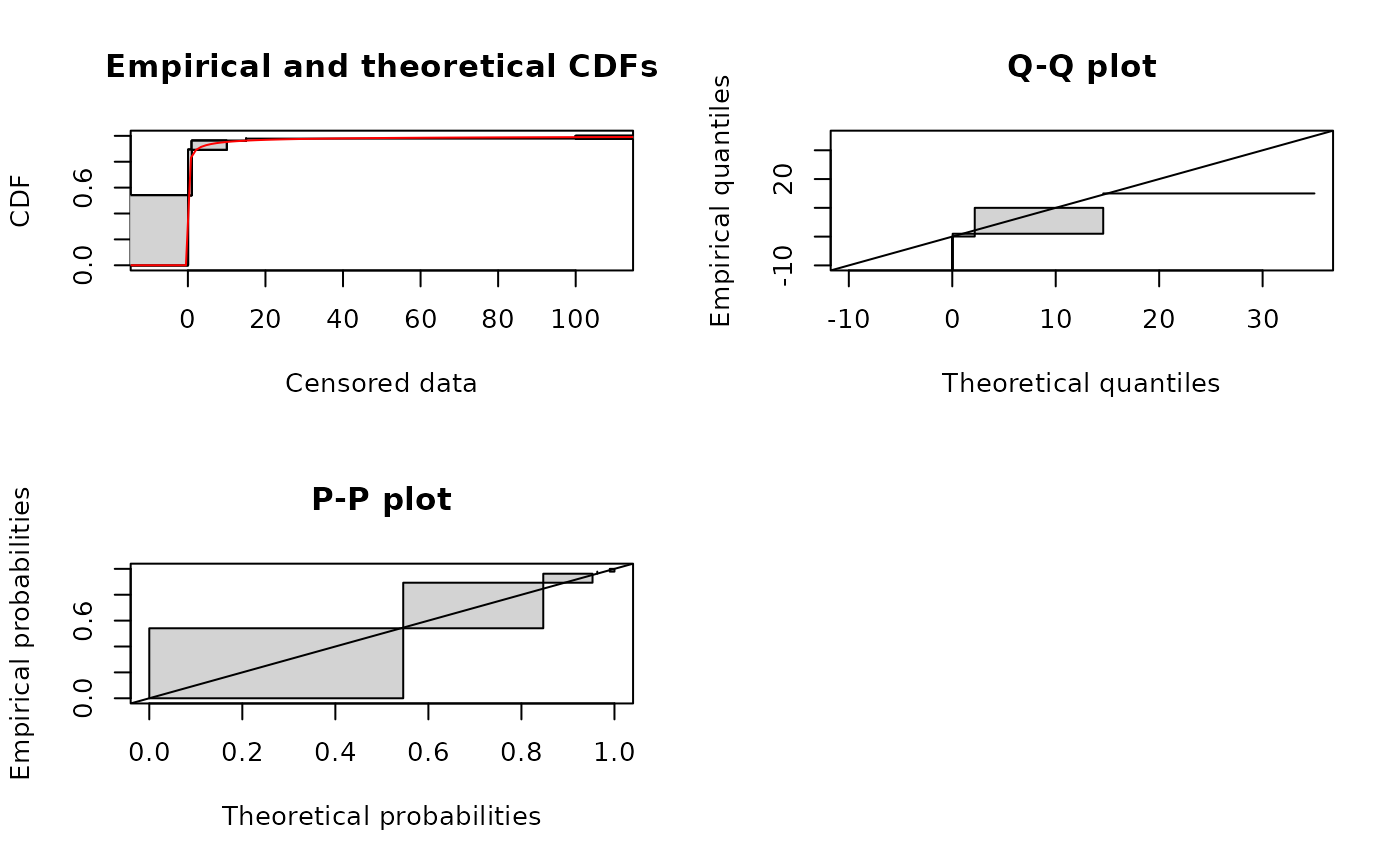
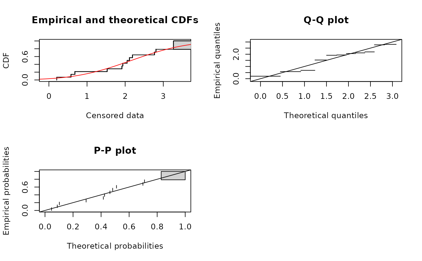
# default plot using the Wang technique (see ?plotdiscens for details)
plot(fitsf)
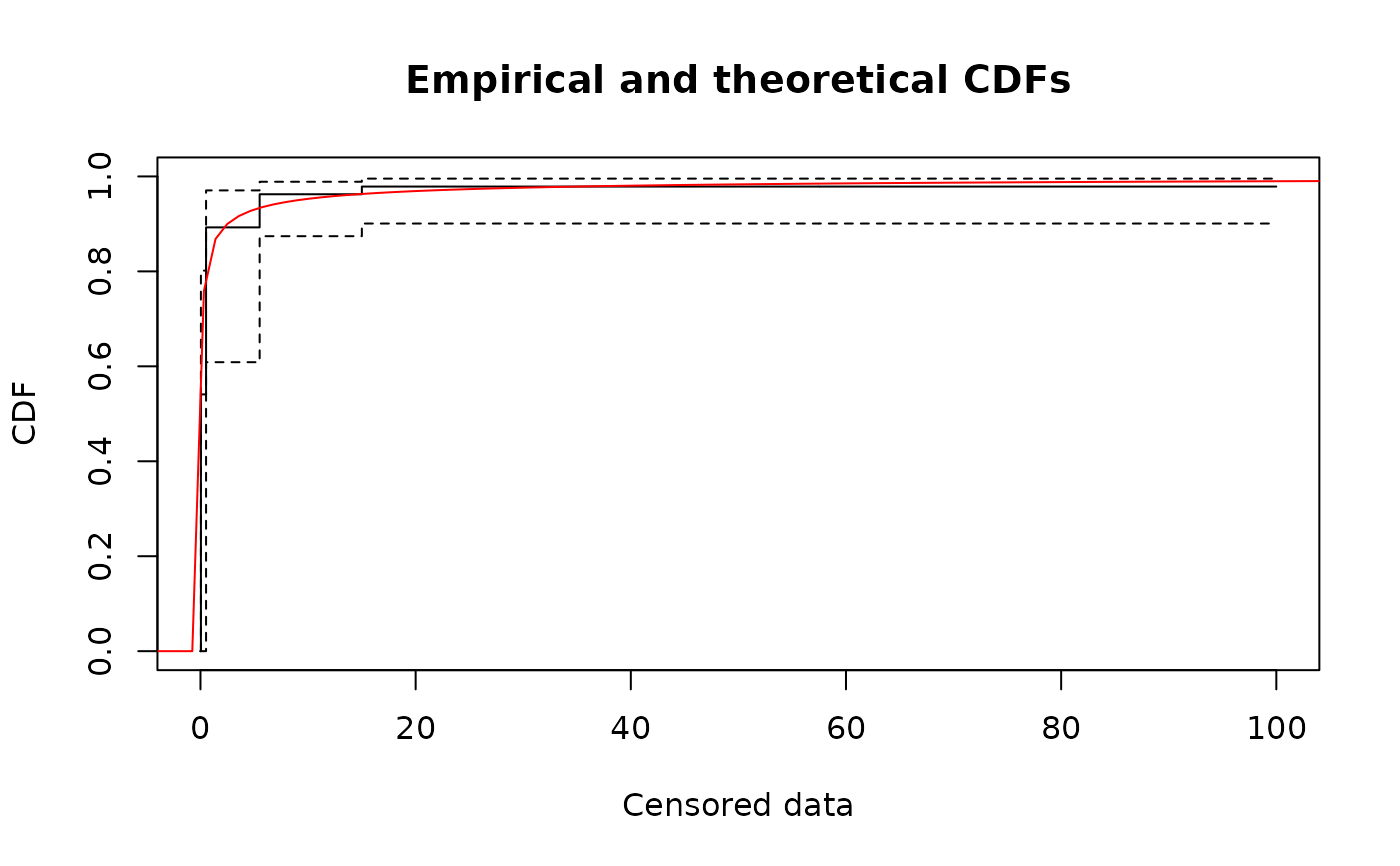
 # plot using the Turnbull algorithm (see ?plotdiscens for details)
# with confidence intervals for the empirical distribution
plot(fitsf, NPMLE = TRUE, NPMLE.method = "Turnbull", Turnbull.confint = TRUE)
#> Warning: Turnbull is now a deprecated option for NPMLE.method. You should use Turnbull.middlepoints
#> of Turnbull.intervals. It was here fixed as Turnbull.middlepoints, equivalent to former Turnbull.
#> Warning: Q-Q plot and P-P plot are available only
#> with the arguments NPMLE.method at Wang (default value) or Turnbull.intervals.
# plot using the Turnbull algorithm (see ?plotdiscens for details)
# with confidence intervals for the empirical distribution
plot(fitsf, NPMLE = TRUE, NPMLE.method = "Turnbull", Turnbull.confint = TRUE)
#> Warning: Turnbull is now a deprecated option for NPMLE.method. You should use Turnbull.middlepoints
#> of Turnbull.intervals. It was here fixed as Turnbull.middlepoints, equivalent to former Turnbull.
#> Warning: Q-Q plot and P-P plot are available only
#> with the arguments NPMLE.method at Wang (default value) or Turnbull.intervals.
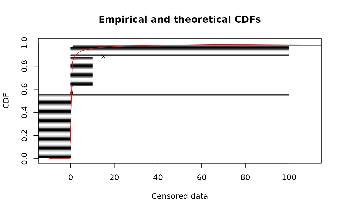
 # basic plot using intervals and points (see ?plotdiscens for details)
plot(fitsf, NPMLE = FALSE)
#> Warning: When NPMLE is FALSE the nonparametric maximum likelihood estimation
#> of the cumulative distribution function is not computed.
#> Q-Q plot and P-P plot are available only with the arguments NPMLE.method at Wang
#> (default value) or Turnbull.intervals.
# basic plot using intervals and points (see ?plotdiscens for details)
plot(fitsf, NPMLE = FALSE)
#> Warning: When NPMLE is FALSE the nonparametric maximum likelihood estimation
#> of the cumulative distribution function is not computed.
#> Q-Q plot and P-P plot are available only with the arguments NPMLE.method at Wang
#> (default value) or Turnbull.intervals.
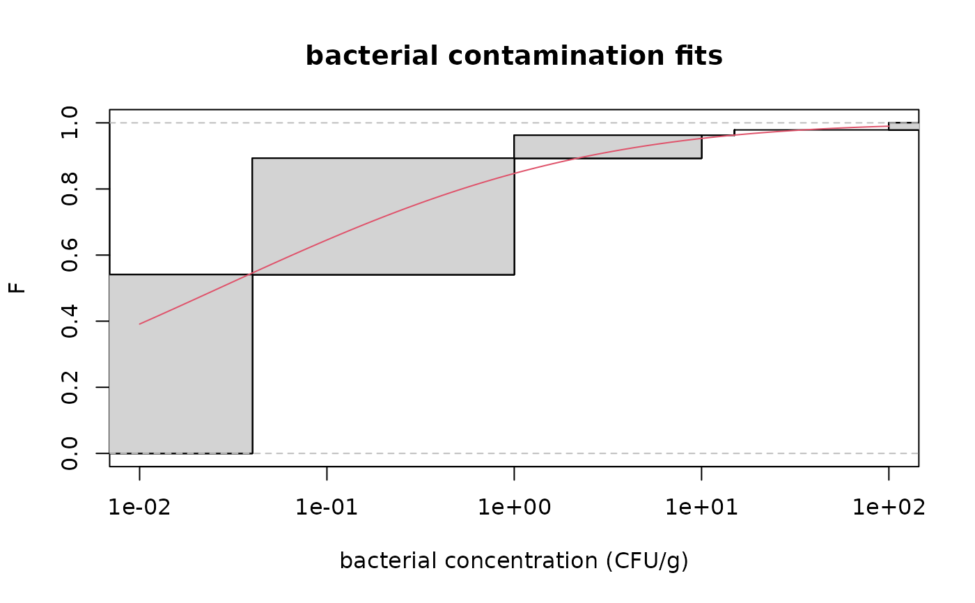
 # plot of the same fit using the Turnbull algorithm in logscale
cdfcompcens(fitsf,main="bacterial contamination fits",
xlab="bacterial concentration (CFU/g)",ylab="F",
addlegend = FALSE,lines01 = TRUE, xlogscale = TRUE, xlim = c(1e-2,1e2))
# plot of the same fit using the Turnbull algorithm in logscale
cdfcompcens(fitsf,main="bacterial contamination fits",
xlab="bacterial concentration (CFU/g)",ylab="F",
addlegend = FALSE,lines01 = TRUE, xlogscale = TRUE, xlim = c(1e-2,1e2))
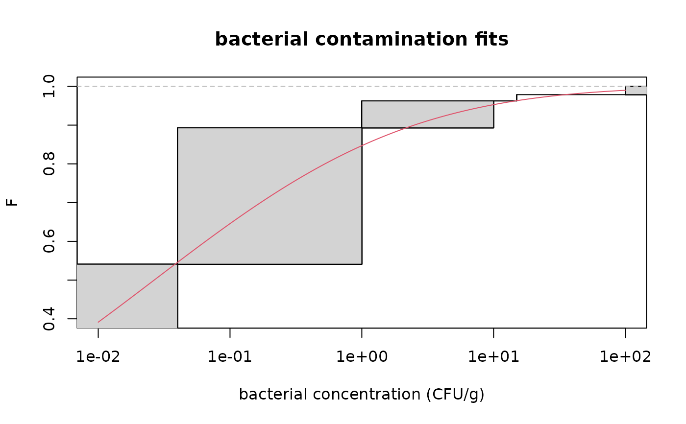
 # zoom on large values of F
cdfcompcens(fitsf,main="bacterial contamination fits",
xlab="bacterial concentration (CFU/g)",ylab="F",
addlegend = FALSE,lines01 = TRUE, xlogscale = TRUE,
xlim = c(1e-2,1e2),ylim=c(0.4,1))
# zoom on large values of F
cdfcompcens(fitsf,main="bacterial contamination fits",
xlab="bacterial concentration (CFU/g)",ylab="F",
addlegend = FALSE,lines01 = TRUE, xlogscale = TRUE,
xlim = c(1e-2,1e2),ylim=c(0.4,1))
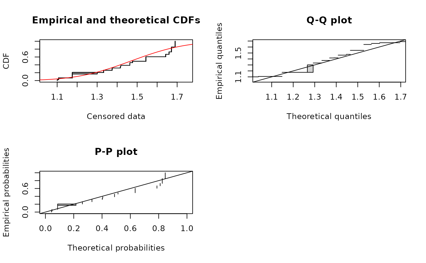
 # (2) Fit of a normal distribution on acute toxicity values
# of fluazinam (in decimal logarithm) for
# macroinvertebrates and zooplancton, using maximum likelihood estimation
# to estimate what is called a species sensitivity distribution
# (SSD) in ecotoxicology
#
data(fluazinam)
log10EC50 <-log10(fluazinam)
fln <- fitdistcens(log10EC50,"norm")
fln
#> Fitting of the distribution ' norm ' on censored data by maximum likelihood
#> Parameters:
#> estimate
#> mean 2.161449
#> sd 1.167290
summary(fln)
#> Fitting of the distribution ' norm ' By maximum likelihood on censored data
#> Parameters
#> estimate Std. Error
#> mean 2.161449 0.3223366
#> sd 1.167290 0.2630390
#> Loglikelihood: -20.41212 AIC: 44.82424 BIC: 46.10235
#> Correlation matrix:
#> mean sd
#> mean 1.0000000 0.1350237
#> sd 0.1350237 1.0000000
#>
plot(fln)
# (2) Fit of a normal distribution on acute toxicity values
# of fluazinam (in decimal logarithm) for
# macroinvertebrates and zooplancton, using maximum likelihood estimation
# to estimate what is called a species sensitivity distribution
# (SSD) in ecotoxicology
#
data(fluazinam)
log10EC50 <-log10(fluazinam)
fln <- fitdistcens(log10EC50,"norm")
fln
#> Fitting of the distribution ' norm ' on censored data by maximum likelihood
#> Parameters:
#> estimate
#> mean 2.161449
#> sd 1.167290
summary(fln)
#> Fitting of the distribution ' norm ' By maximum likelihood on censored data
#> Parameters
#> estimate Std. Error
#> mean 2.161449 0.3223366
#> sd 1.167290 0.2630390
#> Loglikelihood: -20.41212 AIC: 44.82424 BIC: 46.10235
#> Correlation matrix:
#> mean sd
#> mean 1.0000000 0.1350237
#> sd 0.1350237 1.0000000
#>
plot(fln)
 # (3) defining your own distribution functions, here for the Gumbel distribution
# for other distributions, see the CRAN task view dedicated to
# probability distributions
#
dgumbel <- function(x,a,b) 1/b*exp((a-x)/b)*exp(-exp((a-x)/b))
pgumbel <- function(q,a,b) exp(-exp((a-q)/b))
qgumbel <- function(p,a,b) a-b*log(-log(p))
fg <- fitdistcens(log10EC50,"gumbel",start=list(a=1,b=1))
#> Error in checkparamlist(arg_startfix$start.arg, arg_startfix$fix.arg, argddistname, hasnodefaultval): 'start' must specify names which are arguments to 'distr'.
summary(fg)
#> Error: object 'fg' not found
plot(fg)
#> Error: object 'fg' not found
# (4) comparison of fits of various distributions
#
fll <- fitdistcens(log10EC50,"logis")
summary(fll)
#> Fitting of the distribution ' logis ' By maximum likelihood on censored data
#> Parameters
#> estimate Std. Error
#> location 2.1518291 0.3222830
#> scale 0.6910423 0.1745231
#> Loglikelihood: -20.55391 AIC: 45.10781 BIC: 46.38593
#> Correlation matrix:
#> location scale
#> location 1.00000000 0.05097494
#> scale 0.05097494 1.00000000
#>
cdfcompcens(list(fln,fll,fg),legendtext=c("normal","logistic","gumbel"),
xlab = "log10(EC50)")
#> Error: object 'fg' not found
# (5) how to change the optimisation method?
#
fitdistcens(log10EC50,"logis",optim.method="Nelder-Mead")
#> Fitting of the distribution ' logis ' on censored data by maximum likelihood
#> Parameters:
#> estimate
#> location 2.1518291
#> scale 0.6910423
fitdistcens(log10EC50,"logis",optim.method="BFGS")
#> Fitting of the distribution ' logis ' on censored data by maximum likelihood
#> Parameters:
#> estimate
#> location 2.1519961
#> scale 0.6910665
fitdistcens(log10EC50,"logis",optim.method="SANN")
#> Fitting of the distribution ' logis ' on censored data by maximum likelihood
#> Parameters:
#> estimate
#> location 2.0238931
#> scale 0.5261822
# (6) custom optimisation function - example with the genetic algorithm
#
# \donttest{
#wrap genoud function rgenoud package
mygenoud <- function(fn, par, ...)
{
require("rgenoud")
res <- genoud(fn, starting.values=par, ...)
standardres <- c(res, convergence=0)
return(standardres)
}
# call fitdistcens with a 'custom' optimization function
fit.with.genoud <- fitdistcens(log10EC50,"logis", custom.optim=mygenoud, nvars=2,
Domains=cbind(c(0,0), c(5, 5)), boundary.enforcement=1,
print.level=1, hessian=TRUE)
#>
#>
#> Tue Jun 30 14:51:08 2026
#> Domains:
#> 0.000000e+00 <= X1 <= 5.000000e+00
#> 0.000000e+00 <= X2 <= 5.000000e+00
#>
#> Data Type: Floating Point
#> Operators (code number, name, population)
#> (1) Cloning........................... 122
#> (2) Uniform Mutation.................. 125
#> (3) Boundary Mutation................. 125
#> (4) Non-Uniform Mutation.............. 125
#> (5) Polytope Crossover................ 125
#> (6) Simple Crossover.................. 126
#> (7) Whole Non-Uniform Mutation........ 125
#> (8) Heuristic Crossover............... 126
#> (9) Local-Minimum Crossover........... 0
#>
#> HARD Maximum Number of Generations: 100
#> Maximum Nonchanging Generations: 10
#> Population size : 1000
#> Convergence Tolerance: 1.000000e-03
#>
#> Using the BFGS Derivative Based Optimizer on the Best Individual Each Generation.
#> Checking Gradients before Stopping.
#> Not Using Out of Bounds Individuals But Allowing Trespassing.
#>
#> Minimization Problem.
#>
#>
#> Generation# Solution Value
#>
#> 0 1.475558e+00
#> 1 1.468136e+00
#>
#> 'wait.generations' limit reached.
#> No significant improvement in 10 generations.
#>
#> Solution Fitness Value: 1.468136e+00
#>
#> Parameters at the Solution (parameter, gradient):
#>
#> X[ 1] : 2.151910e+00 G[ 1] : -1.894464e-08
#> X[ 2] : 6.909672e-01 G[ 2] : 2.323783e-06
#>
#> Solution Found Generation 1
#> Number of Generations Run 12
#>
#> Tue Jun 30 14:51:09 2026
#> Total run time : 0 hours 0 minutes and 1 seconds
summary(fit.with.genoud)
#> Fitting of the distribution ' logis ' By maximum likelihood on censored data
#> Parameters
#> estimate Std. Error
#> location 2.1519105 0.322257
#> scale 0.6909672 0.174484
#> Loglikelihood: -20.55391 AIC: 45.10781 BIC: 46.38593
#> Correlation matrix:
#> location scale
#> location 1.00000000 0.05106547
#> scale 0.05106547 1.00000000
#>
# }
# (7) estimation of the mean of a normal distribution
# by maximum likelihood with the standard deviation fixed at 1 using the argument fix.arg
#
flnb <- fitdistcens(log10EC50, "norm", start = list(mean = 1),fix.arg = list(sd = 1))
# (8) Fit of a lognormal distribution on acute toxicity values of fluazinam for
# macroinvertebrates and zooplancton, using maximum likelihood estimation
# to estimate what is called a species sensitivity distribution
# (SSD) in ecotoxicology, followed by estimation of the 5 percent quantile value of
# the fitted distribution (which is called the 5 percent hazardous concentration, HC5,
# in ecotoxicology) and estimation of other quantiles.
data(fluazinam)
log10EC50 <-log10(fluazinam)
fln <- fitdistcens(log10EC50,"norm")
quantile(fln, probs = 0.05)
#> Estimated quantiles for each specified probability (censored data)
#> p=0.05
#> estimate 0.2414275
quantile(fln, probs = c(0.05, 0.1, 0.2))
#> Estimated quantiles for each specified probability (censored data)
#> p=0.05 p=0.1 p=0.2
#> estimate 0.2414275 0.6655064 1.179033
# (9) Fit of a lognormal distribution on 72-hour acute salinity tolerance (LC50 values)
# of riverine macro-invertebrates using maximum likelihood estimation
data(salinity)
log10LC50 <-log10(salinity)
fln <- fitdistcens(log10LC50,"norm")
plot(fln)
# (3) defining your own distribution functions, here for the Gumbel distribution
# for other distributions, see the CRAN task view dedicated to
# probability distributions
#
dgumbel <- function(x,a,b) 1/b*exp((a-x)/b)*exp(-exp((a-x)/b))
pgumbel <- function(q,a,b) exp(-exp((a-q)/b))
qgumbel <- function(p,a,b) a-b*log(-log(p))
fg <- fitdistcens(log10EC50,"gumbel",start=list(a=1,b=1))
#> Error in checkparamlist(arg_startfix$start.arg, arg_startfix$fix.arg, argddistname, hasnodefaultval): 'start' must specify names which are arguments to 'distr'.
summary(fg)
#> Error: object 'fg' not found
plot(fg)
#> Error: object 'fg' not found
# (4) comparison of fits of various distributions
#
fll <- fitdistcens(log10EC50,"logis")
summary(fll)
#> Fitting of the distribution ' logis ' By maximum likelihood on censored data
#> Parameters
#> estimate Std. Error
#> location 2.1518291 0.3222830
#> scale 0.6910423 0.1745231
#> Loglikelihood: -20.55391 AIC: 45.10781 BIC: 46.38593
#> Correlation matrix:
#> location scale
#> location 1.00000000 0.05097494
#> scale 0.05097494 1.00000000
#>
cdfcompcens(list(fln,fll,fg),legendtext=c("normal","logistic","gumbel"),
xlab = "log10(EC50)")
#> Error: object 'fg' not found
# (5) how to change the optimisation method?
#
fitdistcens(log10EC50,"logis",optim.method="Nelder-Mead")
#> Fitting of the distribution ' logis ' on censored data by maximum likelihood
#> Parameters:
#> estimate
#> location 2.1518291
#> scale 0.6910423
fitdistcens(log10EC50,"logis",optim.method="BFGS")
#> Fitting of the distribution ' logis ' on censored data by maximum likelihood
#> Parameters:
#> estimate
#> location 2.1519961
#> scale 0.6910665
fitdistcens(log10EC50,"logis",optim.method="SANN")
#> Fitting of the distribution ' logis ' on censored data by maximum likelihood
#> Parameters:
#> estimate
#> location 2.0238931
#> scale 0.5261822
# (6) custom optimisation function - example with the genetic algorithm
#
# \donttest{
#wrap genoud function rgenoud package
mygenoud <- function(fn, par, ...)
{
require("rgenoud")
res <- genoud(fn, starting.values=par, ...)
standardres <- c(res, convergence=0)
return(standardres)
}
# call fitdistcens with a 'custom' optimization function
fit.with.genoud <- fitdistcens(log10EC50,"logis", custom.optim=mygenoud, nvars=2,
Domains=cbind(c(0,0), c(5, 5)), boundary.enforcement=1,
print.level=1, hessian=TRUE)
#>
#>
#> Tue Jun 30 14:51:08 2026
#> Domains:
#> 0.000000e+00 <= X1 <= 5.000000e+00
#> 0.000000e+00 <= X2 <= 5.000000e+00
#>
#> Data Type: Floating Point
#> Operators (code number, name, population)
#> (1) Cloning........................... 122
#> (2) Uniform Mutation.................. 125
#> (3) Boundary Mutation................. 125
#> (4) Non-Uniform Mutation.............. 125
#> (5) Polytope Crossover................ 125
#> (6) Simple Crossover.................. 126
#> (7) Whole Non-Uniform Mutation........ 125
#> (8) Heuristic Crossover............... 126
#> (9) Local-Minimum Crossover........... 0
#>
#> HARD Maximum Number of Generations: 100
#> Maximum Nonchanging Generations: 10
#> Population size : 1000
#> Convergence Tolerance: 1.000000e-03
#>
#> Using the BFGS Derivative Based Optimizer on the Best Individual Each Generation.
#> Checking Gradients before Stopping.
#> Not Using Out of Bounds Individuals But Allowing Trespassing.
#>
#> Minimization Problem.
#>
#>
#> Generation# Solution Value
#>
#> 0 1.475558e+00
#> 1 1.468136e+00
#>
#> 'wait.generations' limit reached.
#> No significant improvement in 10 generations.
#>
#> Solution Fitness Value: 1.468136e+00
#>
#> Parameters at the Solution (parameter, gradient):
#>
#> X[ 1] : 2.151910e+00 G[ 1] : -1.894464e-08
#> X[ 2] : 6.909672e-01 G[ 2] : 2.323783e-06
#>
#> Solution Found Generation 1
#> Number of Generations Run 12
#>
#> Tue Jun 30 14:51:09 2026
#> Total run time : 0 hours 0 minutes and 1 seconds
summary(fit.with.genoud)
#> Fitting of the distribution ' logis ' By maximum likelihood on censored data
#> Parameters
#> estimate Std. Error
#> location 2.1519105 0.322257
#> scale 0.6909672 0.174484
#> Loglikelihood: -20.55391 AIC: 45.10781 BIC: 46.38593
#> Correlation matrix:
#> location scale
#> location 1.00000000 0.05106547
#> scale 0.05106547 1.00000000
#>
# }
# (7) estimation of the mean of a normal distribution
# by maximum likelihood with the standard deviation fixed at 1 using the argument fix.arg
#
flnb <- fitdistcens(log10EC50, "norm", start = list(mean = 1),fix.arg = list(sd = 1))
# (8) Fit of a lognormal distribution on acute toxicity values of fluazinam for
# macroinvertebrates and zooplancton, using maximum likelihood estimation
# to estimate what is called a species sensitivity distribution
# (SSD) in ecotoxicology, followed by estimation of the 5 percent quantile value of
# the fitted distribution (which is called the 5 percent hazardous concentration, HC5,
# in ecotoxicology) and estimation of other quantiles.
data(fluazinam)
log10EC50 <-log10(fluazinam)
fln <- fitdistcens(log10EC50,"norm")
quantile(fln, probs = 0.05)
#> Estimated quantiles for each specified probability (censored data)
#> p=0.05
#> estimate 0.2414275
quantile(fln, probs = c(0.05, 0.1, 0.2))
#> Estimated quantiles for each specified probability (censored data)
#> p=0.05 p=0.1 p=0.2
#> estimate 0.2414275 0.6655064 1.179033
# (9) Fit of a lognormal distribution on 72-hour acute salinity tolerance (LC50 values)
# of riverine macro-invertebrates using maximum likelihood estimation
data(salinity)
log10LC50 <-log10(salinity)
fln <- fitdistcens(log10LC50,"norm")
plot(fln)