Goodness-of-fit statistics
gofstat.RdComputes goodness-of-fit statistics for parametric distributions fitted to a same censored or non-censored data set.
Arguments
- f
An object of class
"fitdist"(or"fitdistcens"), output of the functionfitdist()(resp."fitdist()"), or a list of"fitdist"objects, or a list of"fitdistcens"objects.- chisqbreaks
Only usable for non censored data, a numeric vector defining the breaks of the cells used to compute the chi-squared statistic. If omitted, these breaks are automatically computed from the data in order to reach roughly the same number of observations per cell, roughly equal to the argument
meancount, or sligthly more if there are some ties.- meancount
Only usable for non censored data, the mean number of observations per cell expected for the definition of the breaks of the cells used to compute the chi-squared statistic. This argument will not be taken into account if the breaks are directly defined in the argument
chisqbreaks. Ifchisqbreaksandmeancountare both omitted,meancountis fixed in order to obtain roughly \((4n)^{2/5}\) cells with \(n\) the length of the dataset.- discrete
If
TRUE, only the Chi-squared statistic and information criteria are computed. If missing,discreteis passed from the first object of class"fitdist"of the listf. For censored data this argument is ignored, as censored data are considered continuous.- fitnames
A vector defining the names of the fits.
- x
An object of class
"gofstat.fitdist"or"gofstat.fitdistcens".- ...
Further arguments to be passed to generic functions.
Details
For any type of data (censored or not), information criteria are calculated. For non censored data, added Goodness-of-fit statistics are computed as described below.
The Chi-squared statistic is computed using cells defined
by the argument
chisqbreaks or cells automatically defined from data, in order
to reach roughly the same number of observations per cell, roughly equal to the argument
meancount, or sligthly more if there are some ties.
The choice to define cells from the empirical distribution (data), and not from the
theoretical distribution, was done to enable the comparison of Chi-squared values obtained
with different distributions fitted on a same data set.
If chisqbreaks and meancount
are both omitted, meancount is fixed in order to obtain roughly \((4n)^{2/5}\) cells,
with \(n\) the length of the data set (Vose, 2000).
The Chi-squared statistic is not computed if the program fails
to define enough cells due to a too small dataset. When the Chi-squared statistic is computed,
and if the degree of freedom (nb of cells - nb of parameters - 1) of the corresponding distribution
is strictly positive, the p-value of the Chi-squared test is returned.
For continuous distributions, Kolmogorov-Smirnov, Cramer-von Mises and Anderson-Darling and statistics are also computed, as defined by Stephens (1986).
An approximate Kolmogorov-Smirnov test is performed by assuming the distribution parameters known. The critical value defined by Stephens (1986) for a completely specified distribution is used to reject or not the distribution at the significance level 0.05. Because of this approximation, the result of the test (decision of rejection of the distribution or not) is returned only for data sets with more than 30 observations. Note that this approximate test may be too conservative.
For data sets with more than 5 observations and for distributions for
which the test is described by Stephens (1986) for maximum likelihood estimations
("exp", "cauchy", "gamma" and "weibull"),
the Cramer-von Mises and Anderson-darling tests are performed as described by Stephens (1986).
Those tests take into
account the fact that the parameters are not known but estimated from the data by maximum likelihood.
The result is the
decision to reject or not the distribution at the significance level 0.05. Those tests are available
only for maximum likelihood estimations.
Only recommended statistics are automatically printed, i.e.
Cramer-von Mises, Anderson-Darling and Kolmogorov statistics for continuous distributions and
Chi-squared statistics for discrete ones ( "binom",
"nbinom", "geom", "hyper" and "pois" ).
Results of the tests are not printed but stored in the output of the function.
Value
gofstat() returns an object of class "gofstat.fitdist" or "gofstat.fitdistcens" with following components or a sublist of them (only aic, bic and nbfit for censored data) ,
- chisq
a named vector with the Chi-squared statistics or
NULLif not computed- chisqbreaks
common breaks used to define cells in the Chi-squared statistic
- chisqpvalue
a named vector with the p-values of the Chi-squared statistic or
NULLif not computed- chisqdf
a named vector with the degrees of freedom of the Chi-squared distribution or
NULLif not computed- chisqtable
a table with observed and theoretical counts used for the Chi-squared calculations
- cvm
a named vector of the Cramer-von Mises statistics or
"not computed"if not computed- cvmtest
a named vector of the decisions of the Cramer-von Mises test or
"not computed"if not computed- ad
a named vector with the Anderson-Darling statistics or
"not computed"if not computed- adtest
a named vector with the decisions of the Anderson-Darling test or
"not computed"if not computed- ks
a named vector with the Kolmogorov-Smirnov statistic or
"not computed"if not computed- kstest
a named vector with the decisions of the Kolmogorov-Smirnov test or
"not computed"if not computed- aic
a named vector with the values of the Akaike's Information Criterion.
- bic
a named vector with the values of the Bayesian Information Criterion.
- discrete
the input argument or the automatic definition by the function from the first object of class
"fitdist"of the list in input.- nbfit
Number of fits in argument.
See also
See fitdist.
Please visit the Frequently Asked Questions.
References
Cullen AC and Frey HC (1999), Probabilistic techniques in exposure assessment. Plenum Press, USA, pp. 81-155.
Stephens MA (1986), Tests based on edf statistics. In Goodness-of-fit techniques (D'Agostino RB and Stephens MA, eds), Marcel Dekker, New York, pp. 97-194.
Venables WN and Ripley BD (2002), Modern applied statistics with S. Springer, New York, pp. 435-446, doi:10.1007/978-0-387-21706-2 .
Vose D (2000), Risk analysis, a quantitative guide. John Wiley & Sons Ltd, Chischester, England, pp. 99-143.
Delignette-Muller ML and Dutang C (2015), fitdistrplus: An R Package for Fitting Distributions. Journal of Statistical Software, 64(4), 1-34, doi:10.18637/jss.v064.i04 .
Examples
set.seed(123) # here just to make random sampling reproducible
# (1) fit of two distributions to the serving size data
# by maximum likelihood estimation
# and comparison of goodness-of-fit statistics
#
data(groundbeef)
serving <- groundbeef$serving
(fitg <- fitdist(serving, "gamma"))
#> Fitting of the distribution ' gamma ' by maximum likelihood
#> Parameters:
#> estimate Std. Error
#> shape 4.00955898 0.341451640
#> rate 0.05443907 0.004937239
gofstat(fitg)
#> Goodness-of-fit statistics
#> 1-mle-gamma
#> Kolmogorov-Smirnov statistic 0.1281486
#> Cramer-von Mises statistic 0.6936274
#> Anderson-Darling statistic 3.5672625
#>
#> Goodness-of-fit criteria
#> 1-mle-gamma
#> Akaike's Information Criterion 2511.250
#> Bayesian Information Criterion 2518.325
(fitln <- fitdist(serving, "lnorm"))
#> Fitting of the distribution ' lnorm ' by maximum likelihood
#> Parameters:
#> estimate Std. Error
#> meanlog 4.1693701 0.03366988
#> sdlog 0.5366095 0.02380783
gofstat(fitln)
#> Goodness-of-fit statistics
#> 1-mle-lnorm
#> Kolmogorov-Smirnov statistic 0.1493090
#> Cramer-von Mises statistic 0.8277358
#> Anderson-Darling statistic 4.5436542
#>
#> Goodness-of-fit criteria
#> 1-mle-lnorm
#> Akaike's Information Criterion 2526.639
#> Bayesian Information Criterion 2533.713
gofstat(list(fitg, fitln))
#> Goodness-of-fit statistics
#> 1-mle-gamma 2-mle-lnorm
#> Kolmogorov-Smirnov statistic 0.1281486 0.1493090
#> Cramer-von Mises statistic 0.6936274 0.8277358
#> Anderson-Darling statistic 3.5672625 4.5436542
#>
#> Goodness-of-fit criteria
#> 1-mle-gamma 2-mle-lnorm
#> Akaike's Information Criterion 2511.250 2526.639
#> Bayesian Information Criterion 2518.325 2533.713
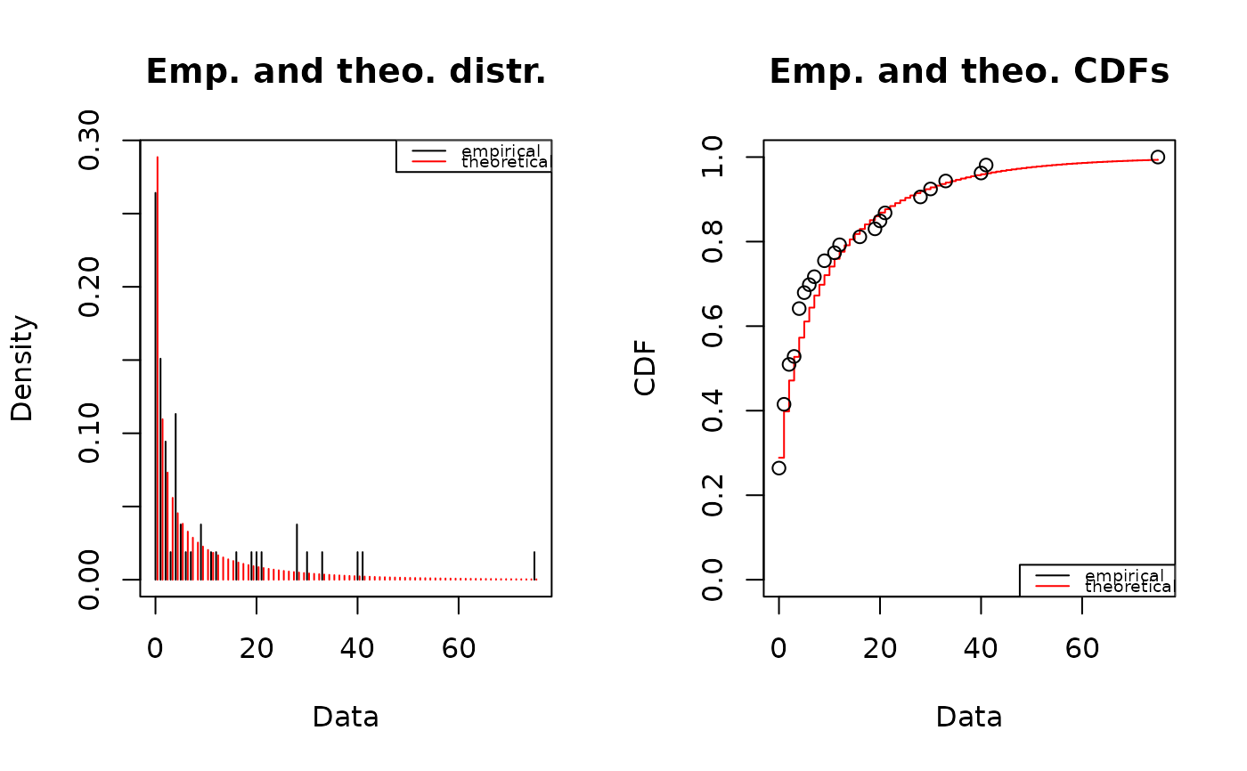
# (2) fit of two discrete distributions to toxocara data
# and comparison of goodness-of-fit statistics
#
data(toxocara)
number <- toxocara$number
fitp <- fitdist(number,"pois")
summary(fitp)
#> Fitting of the distribution ' pois ' by maximum likelihood
#> Parameters :
#> estimate Std. Error
#> lambda 8.679245 0.4046719
#> Loglikelihood: -507.5334 AIC: 1017.067 BIC: 1019.037
plot(fitp)
 fitnb <- fitdist(number,"nbinom")
summary(fitnb)
#> Fitting of the distribution ' nbinom ' by maximum likelihood
#> Parameters :
#> estimate Std. Error
#> size 0.3971457 0.08289027
#> mu 8.6802520 1.93501002
#> Loglikelihood: -159.3441 AIC: 322.6882 BIC: 326.6288
#> Correlation matrix:
#> size mu
#> size 1.000000000 -0.000103854
#> mu -0.000103854 1.000000000
#>
plot(fitnb)
fitnb <- fitdist(number,"nbinom")
summary(fitnb)
#> Fitting of the distribution ' nbinom ' by maximum likelihood
#> Parameters :
#> estimate Std. Error
#> size 0.3971457 0.08289027
#> mu 8.6802520 1.93501002
#> Loglikelihood: -159.3441 AIC: 322.6882 BIC: 326.6288
#> Correlation matrix:
#> size mu
#> size 1.000000000 -0.000103854
#> mu -0.000103854 1.000000000
#>
plot(fitnb)
 gofstat(list(fitp, fitnb),fitnames = c("Poisson","negbin"))
#> Chi-squared statistic: 31256.96 7.48606
#> Degree of freedom of the Chi-squared distribution: 5 4
#> Chi-squared p-value: 0 0.1123255
#> the p-value may be wrong with some theoretical counts < 5
#> Chi-squared table:
#> obscounts theo Poisson theo negbin
#> <= 0 14 0.009014207 15.295027
#> <= 1 8 0.078236515 5.808596
#> <= 3 6 1.321767253 6.845015
#> <= 4 6 2.131297825 2.407815
#> <= 9 6 29.827829425 7.835196
#> <= 21 6 19.626223437 8.271110
#> > 21 7 0.005631338 6.537242
#>
#> Goodness-of-fit criteria
#> Poisson negbin
#> Akaike's Information Criterion 1017.067 322.6882
#> Bayesian Information Criterion 1019.037 326.6288
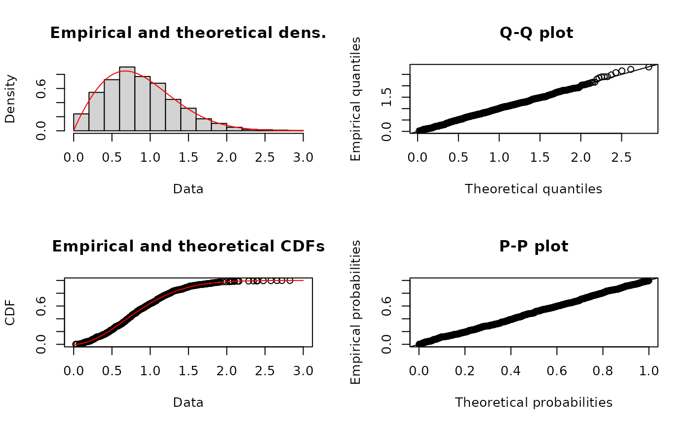
# (3) Get Chi-squared results in addition to
# recommended statistics for continuous distributions
#
x4 <- rweibull(n=1000,shape=2,scale=1)
# fit of the good distribution
f4 <- fitdist(x4,"weibull")
plot(f4)
gofstat(list(fitp, fitnb),fitnames = c("Poisson","negbin"))
#> Chi-squared statistic: 31256.96 7.48606
#> Degree of freedom of the Chi-squared distribution: 5 4
#> Chi-squared p-value: 0 0.1123255
#> the p-value may be wrong with some theoretical counts < 5
#> Chi-squared table:
#> obscounts theo Poisson theo negbin
#> <= 0 14 0.009014207 15.295027
#> <= 1 8 0.078236515 5.808596
#> <= 3 6 1.321767253 6.845015
#> <= 4 6 2.131297825 2.407815
#> <= 9 6 29.827829425 7.835196
#> <= 21 6 19.626223437 8.271110
#> > 21 7 0.005631338 6.537242
#>
#> Goodness-of-fit criteria
#> Poisson negbin
#> Akaike's Information Criterion 1017.067 322.6882
#> Bayesian Information Criterion 1019.037 326.6288
# (3) Get Chi-squared results in addition to
# recommended statistics for continuous distributions
#
x4 <- rweibull(n=1000,shape=2,scale=1)
# fit of the good distribution
f4 <- fitdist(x4,"weibull")
plot(f4)
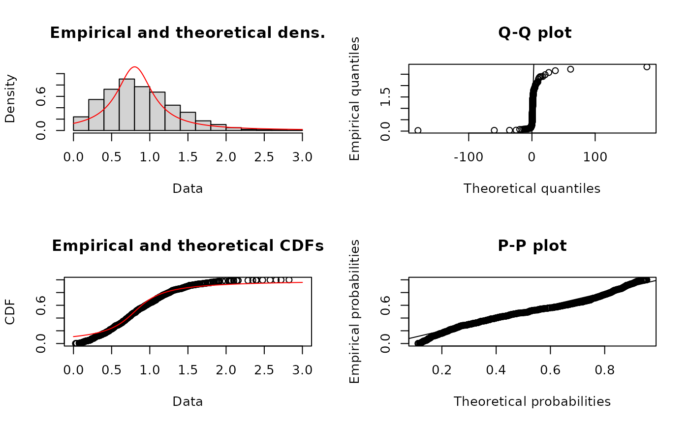
 # fit of a bad distribution
f4b <- fitdist(x4,"cauchy")
plot(f4b)
# fit of a bad distribution
f4b <- fitdist(x4,"cauchy")
plot(f4b)
 (g <- gofstat(list(f4,f4b),fitnames=c("Weibull", "Cauchy")))
#> Goodness-of-fit statistics
#> Weibull Cauchy
#> Kolmogorov-Smirnov statistic 0.01037199 0.1132388
#> Cramer-von Mises statistic 0.01339266 1.8983088
#> Anderson-Darling statistic 0.10469400 18.3876581
#>
#> Goodness-of-fit criteria
#> Weibull Cauchy
#> Akaike's Information Criterion 1191.304 1653.580
#> Bayesian Information Criterion 1201.120 1663.396
g$chisq
#> Weibull Cauchy
#> 17.92108 303.30862
g$chisqdf
#> Weibull Cauchy
#> 25 25
g$chisqpvalue
#> Weibull Cauchy
#> 8.457227e-01 1.303089e-49
g$chisqtable
#> obscounts theo Weibull theo Cauchy
#> <= 0.1919 36 34.91742 135.05298
#> <= 0.2867 36 41.83188 20.66766
#> <= 0.344 36 32.09826 15.51837
#> <= 0.3971 36 33.83042 17.10364
#> <= 0.4558 36 41.24895 22.70295
#> <= 0.4955 36 29.83167 18.13700
#> <= 0.5418 36 36.40602 24.59362
#> <= 0.587 36 36.92018 28.24427
#> <= 0.6293 36 35.41350 30.72730
#> <= 0.6663 36 31.47754 30.61845
#> <= 0.719 36 45.08380 49.47567
#> <= 0.7561 36 31.80740 38.61825
#> <= 0.7992 36 36.74604 47.54081
#> <= 0.8464 36 39.57486 52.96082
#> <= 0.8877 36 33.89411 45.01908
#> <= 0.9375 36 39.73567 50.32862
#> <= 0.9767 36 30.27225 35.56734
#> <= 1.02 36 31.82911 34.31234
#> <= 1.07 36 35.72927 34.62020
#> <= 1.124 36 35.66262 30.64482
#> <= 1.184 36 37.14216 28.21807
#> <= 1.239 36 31.25428 21.24728
#> <= 1.344 36 51.55358 31.10538
#> <= 1.408 36 26.67113 14.65142
#> <= 1.514 36 37.24750 19.48295
#> <= 1.664 36 38.85680 20.21006
#> <= 1.891 36 34.98981 20.60987
#> > 1.891 28 27.97378 82.02081
# and by defining the breaks
(g <- gofstat(list(f4,f4b),
chisqbreaks = seq(from = min(x4), to = max(x4), length.out = 10), fitnames=c("Weibull", "Cauchy")))
#> Goodness-of-fit statistics
#> Weibull Cauchy
#> Kolmogorov-Smirnov statistic 0.01037199 0.1132388
#> Cramer-von Mises statistic 0.01339266 1.8983088
#> Anderson-Darling statistic 0.10469400 18.3876581
#>
#> Goodness-of-fit criteria
#> Weibull Cauchy
#> Akaike's Information Criterion 1191.304 1653.580
#> Bayesian Information Criterion 1201.120 1663.396
g$chisq
#> Weibull Cauchy
#> 3.782153 297.252189
g$chisqdf
#> Weibull Cauchy
#> 8 8
g$chisqpvalue
#> Weibull Cauchy
#> 8.762240e-01 1.582838e-59
g$chisqtable
#> obscounts theo Weibull theo Cauchy
#> <= 0.02441 1 0.5565072 108.969476
#> <= 0.3295 93 99.7034224 58.075483
#> <= 0.6345 233 226.6667705 149.817012
#> <= 0.9396 252 255.5506853 312.466336
#> <= 1.245 214 203.0083829 184.383134
#> <= 1.55 120 123.3077145 68.910097
#> <= 1.855 57 59.1360492 32.625213
#> <= 2.16 19 22.7494898 18.641871
#> <= 2.465 8 7.0827885 11.985162
#> <= 2.77 3 1.7943360 8.332061
#> > 2.77 0 0.4438538 45.794155
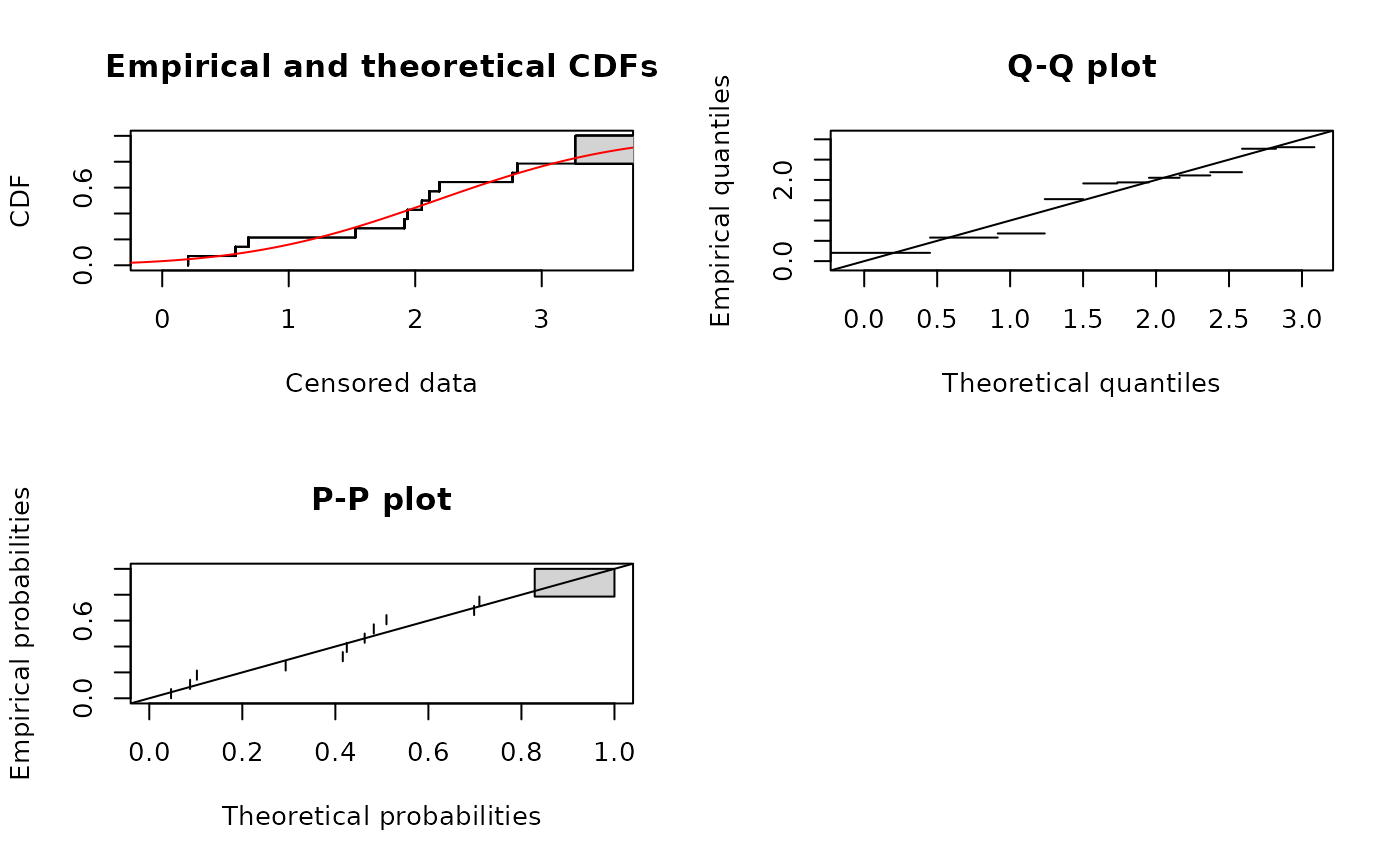
# (4) fit of two distributions on acute toxicity values
# of fluazinam (in decimal logarithm) for
# macroinvertebrates and zooplancton
# and comparison of goodness-of-fit statistics
#
data(fluazinam)
log10EC50 <-log10(fluazinam)
(fln <- fitdistcens(log10EC50,"norm"))
#> Fitting of the distribution ' norm ' on censored data by maximum likelihood
#> Parameters:
#> estimate
#> mean 2.161449
#> sd 1.167290
plot(fln)
(g <- gofstat(list(f4,f4b),fitnames=c("Weibull", "Cauchy")))
#> Goodness-of-fit statistics
#> Weibull Cauchy
#> Kolmogorov-Smirnov statistic 0.01037199 0.1132388
#> Cramer-von Mises statistic 0.01339266 1.8983088
#> Anderson-Darling statistic 0.10469400 18.3876581
#>
#> Goodness-of-fit criteria
#> Weibull Cauchy
#> Akaike's Information Criterion 1191.304 1653.580
#> Bayesian Information Criterion 1201.120 1663.396
g$chisq
#> Weibull Cauchy
#> 17.92108 303.30862
g$chisqdf
#> Weibull Cauchy
#> 25 25
g$chisqpvalue
#> Weibull Cauchy
#> 8.457227e-01 1.303089e-49
g$chisqtable
#> obscounts theo Weibull theo Cauchy
#> <= 0.1919 36 34.91742 135.05298
#> <= 0.2867 36 41.83188 20.66766
#> <= 0.344 36 32.09826 15.51837
#> <= 0.3971 36 33.83042 17.10364
#> <= 0.4558 36 41.24895 22.70295
#> <= 0.4955 36 29.83167 18.13700
#> <= 0.5418 36 36.40602 24.59362
#> <= 0.587 36 36.92018 28.24427
#> <= 0.6293 36 35.41350 30.72730
#> <= 0.6663 36 31.47754 30.61845
#> <= 0.719 36 45.08380 49.47567
#> <= 0.7561 36 31.80740 38.61825
#> <= 0.7992 36 36.74604 47.54081
#> <= 0.8464 36 39.57486 52.96082
#> <= 0.8877 36 33.89411 45.01908
#> <= 0.9375 36 39.73567 50.32862
#> <= 0.9767 36 30.27225 35.56734
#> <= 1.02 36 31.82911 34.31234
#> <= 1.07 36 35.72927 34.62020
#> <= 1.124 36 35.66262 30.64482
#> <= 1.184 36 37.14216 28.21807
#> <= 1.239 36 31.25428 21.24728
#> <= 1.344 36 51.55358 31.10538
#> <= 1.408 36 26.67113 14.65142
#> <= 1.514 36 37.24750 19.48295
#> <= 1.664 36 38.85680 20.21006
#> <= 1.891 36 34.98981 20.60987
#> > 1.891 28 27.97378 82.02081
# and by defining the breaks
(g <- gofstat(list(f4,f4b),
chisqbreaks = seq(from = min(x4), to = max(x4), length.out = 10), fitnames=c("Weibull", "Cauchy")))
#> Goodness-of-fit statistics
#> Weibull Cauchy
#> Kolmogorov-Smirnov statistic 0.01037199 0.1132388
#> Cramer-von Mises statistic 0.01339266 1.8983088
#> Anderson-Darling statistic 0.10469400 18.3876581
#>
#> Goodness-of-fit criteria
#> Weibull Cauchy
#> Akaike's Information Criterion 1191.304 1653.580
#> Bayesian Information Criterion 1201.120 1663.396
g$chisq
#> Weibull Cauchy
#> 3.782153 297.252189
g$chisqdf
#> Weibull Cauchy
#> 8 8
g$chisqpvalue
#> Weibull Cauchy
#> 8.762240e-01 1.582838e-59
g$chisqtable
#> obscounts theo Weibull theo Cauchy
#> <= 0.02441 1 0.5565072 108.969476
#> <= 0.3295 93 99.7034224 58.075483
#> <= 0.6345 233 226.6667705 149.817012
#> <= 0.9396 252 255.5506853 312.466336
#> <= 1.245 214 203.0083829 184.383134
#> <= 1.55 120 123.3077145 68.910097
#> <= 1.855 57 59.1360492 32.625213
#> <= 2.16 19 22.7494898 18.641871
#> <= 2.465 8 7.0827885 11.985162
#> <= 2.77 3 1.7943360 8.332061
#> > 2.77 0 0.4438538 45.794155
# (4) fit of two distributions on acute toxicity values
# of fluazinam (in decimal logarithm) for
# macroinvertebrates and zooplancton
# and comparison of goodness-of-fit statistics
#
data(fluazinam)
log10EC50 <-log10(fluazinam)
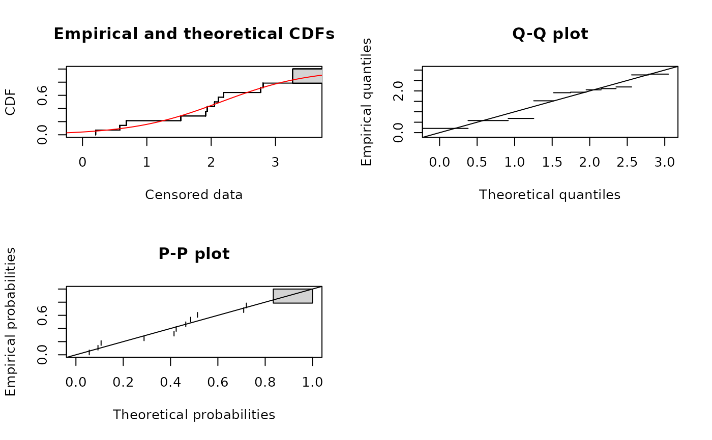
(fln <- fitdistcens(log10EC50,"norm"))
#> Fitting of the distribution ' norm ' on censored data by maximum likelihood
#> Parameters:
#> estimate
#> mean 2.161449
#> sd 1.167290
plot(fln)
 gofstat(fln)
#>
#> Goodness-of-fit criteria
#> 1-mle-norm
#> Akaike's Information Criterion 44.82424
#> Bayesian Information Criterion 46.10235
(fll <- fitdistcens(log10EC50,"logis"))
#> Fitting of the distribution ' logis ' on censored data by maximum likelihood
#> Parameters:
#> estimate
#> location 2.1518291
#> scale 0.6910423
plot(fll)
gofstat(fln)
#>
#> Goodness-of-fit criteria
#> 1-mle-norm
#> Akaike's Information Criterion 44.82424
#> Bayesian Information Criterion 46.10235
(fll <- fitdistcens(log10EC50,"logis"))
#> Fitting of the distribution ' logis ' on censored data by maximum likelihood
#> Parameters:
#> estimate
#> location 2.1518291
#> scale 0.6910423
plot(fll)
 gofstat(fll)
#>
#> Goodness-of-fit criteria
#> 1-mle-logis
#> Akaike's Information Criterion 45.10781
#> Bayesian Information Criterion 46.38593
gofstat(list(fll, fln), fitnames = c("loglogistic", "lognormal"))
#>
#> Goodness-of-fit criteria
#> loglogistic lognormal
#> Akaike's Information Criterion 45.10781 44.82424
#> Bayesian Information Criterion 46.38593 46.10235
gofstat(fll)
#>
#> Goodness-of-fit criteria
#> 1-mle-logis
#> Akaike's Information Criterion 45.10781
#> Bayesian Information Criterion 46.38593
gofstat(list(fll, fln), fitnames = c("loglogistic", "lognormal"))
#>
#> Goodness-of-fit criteria
#> loglogistic lognormal
#> Akaike's Information Criterion 45.10781 44.82424
#> Bayesian Information Criterion 46.38593 46.10235