Species Sensitivity Distribution (SSD) for endosulfan

Summary of 48- to 96-hour acute toxicity values (LC50 and EC50 values) for exposure of Australian an Non-Australian taxa to endosulfan.

Usage

data(endosulfan)

Format

endosulfan is a data frame with 4 columns, named ATV for Acute Toxicity Value (geometric mean of LC50 ou EC50 values in micrograms per liter), Australian (coding for Australian or another origin), group (arthropods, fish or non-arthropod invertebrates) and taxa.

Source

Hose, G.C., Van den Brink, P.J. 2004. Confirming the Species-Sensitivity Distribution Concept for Endosulfan Using Laboratory, Mesocosms, and Field Data. Archives of Environmental Contamination and Toxicology, 47, 511-520.

Examples

# (1) load of data
#
data(endosulfan)

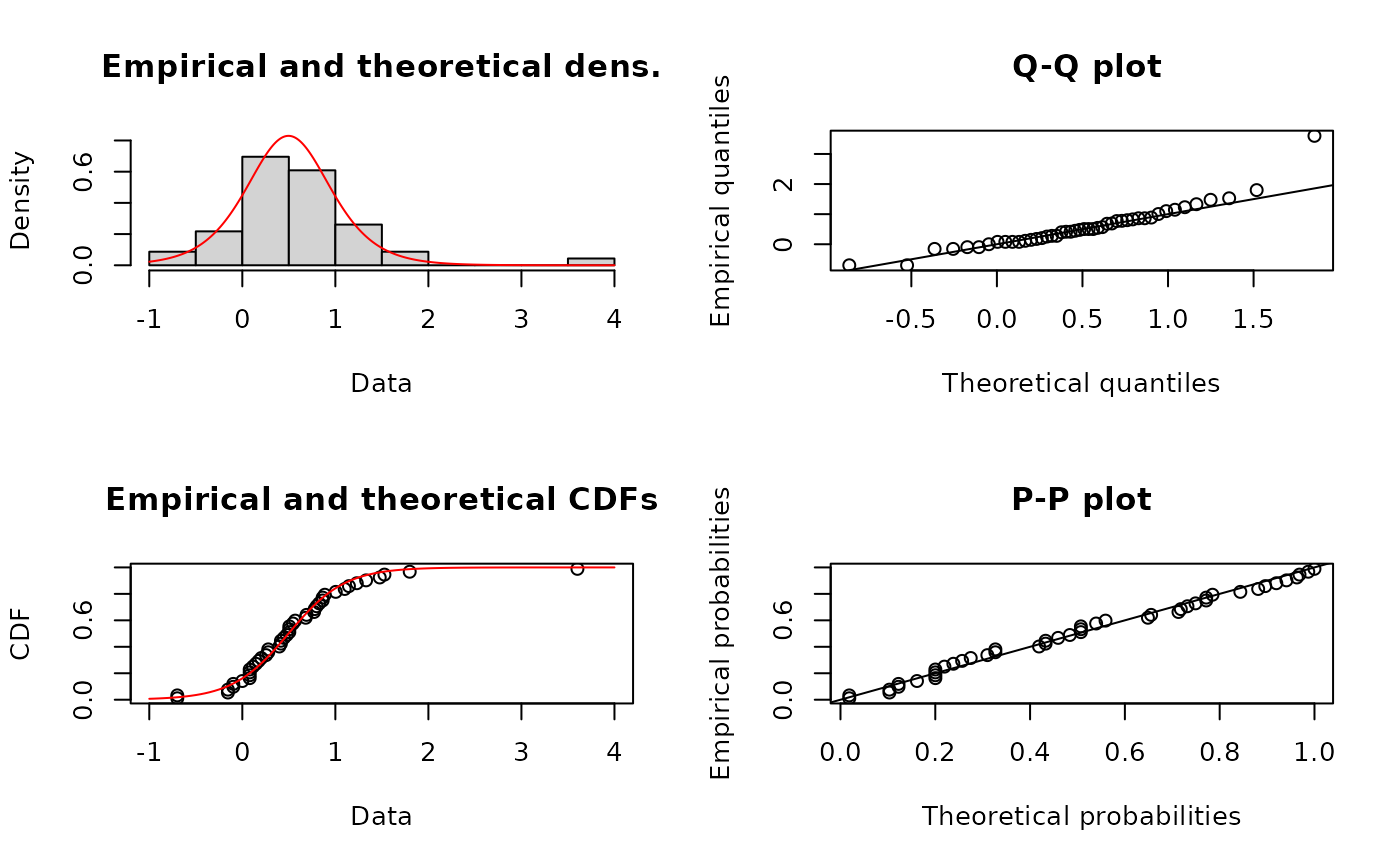
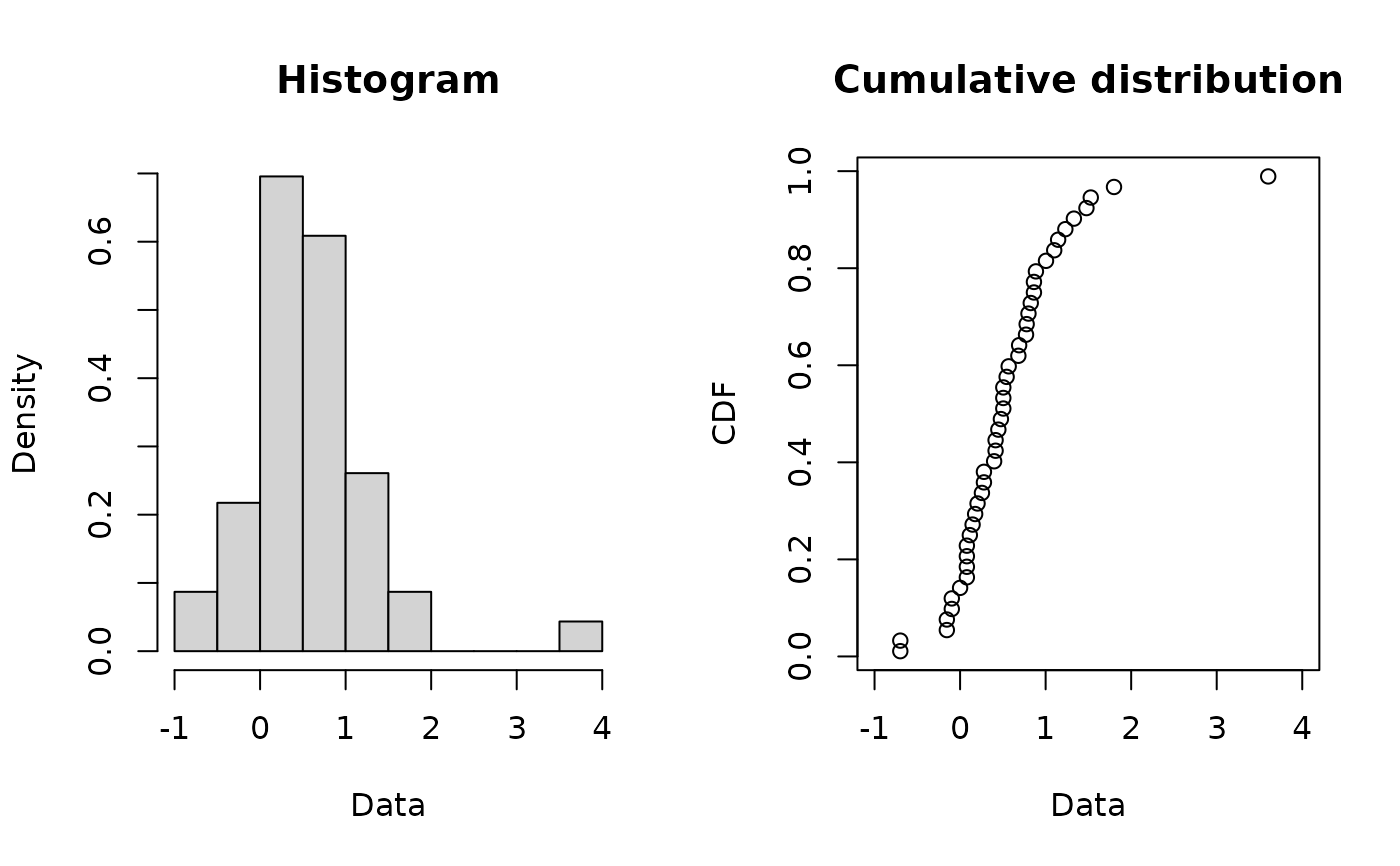
# (2) plot and description of data for non Australian fish in decimal logarithm
#
log10ATV <-log10(subset(endosulfan,(Australian == "no") & (group == "Fish"))$ATV)
plotdist(log10ATV)

descdist(log10ATV,boot=11)

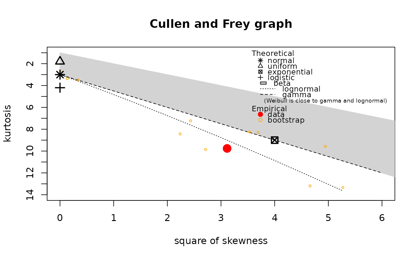#> summary statistics
#> ------
#> min:  -0.69897   max:  3.60206 
#> median:  0.4911356 
#> mean:  0.5657595 
#> estimated sd:  0.7034928 
#> estimated skewness:  1.764601 
#> estimated kurtosis:  9.759505 

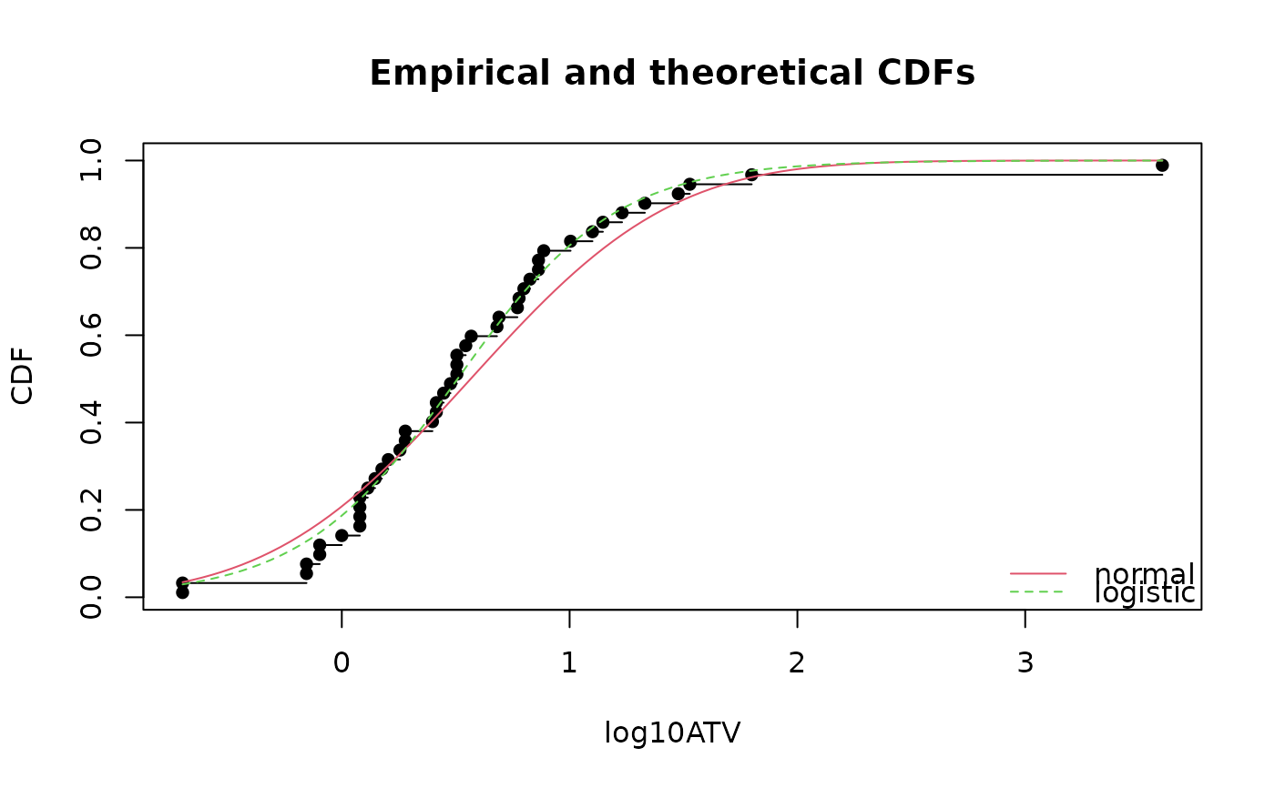
# (3) fit of a normal and a logistic distribution to data in log10
# (classical distributions used for SSD)
# and visual comparison of the fits
#
fln <- fitdist(log10ATV,"norm")
summary(fln)
#> Fitting of the distribution ' norm ' by maximum likelihood 
#> Parameters : 
#>       estimate Std. Error
#> mean 0.5657595  0.6958041
#> sd   0.6958041  0.4920032
#> Loglikelihood:  -48.58757   AIC:  101.1751   BIC:  104.8324 
#> Correlation matrix:
#>      mean sd
#> mean    1  0
#> sd      0  1
#> 

fll <- fitdist(log10ATV,"logis")
summary(fll)
#> Fitting of the distribution ' logis ' by maximum likelihood 
#> Parameters : 
#>           estimate Std. Error
#> location 0.5082818  0.5901708
#> scale    0.3457256  0.2917097
#> Loglikelihood:  -44.31825   AIC:  92.6365   BIC:  96.29378 
#> Correlation matrix:
#>            location      scale
#> location 1.00000000 0.04028287
#> scale    0.04028287 1.00000000
#> 

cdfcomp(list(fln,fll),legendtext=c("normal","logistic"),
xlab="log10ATV")


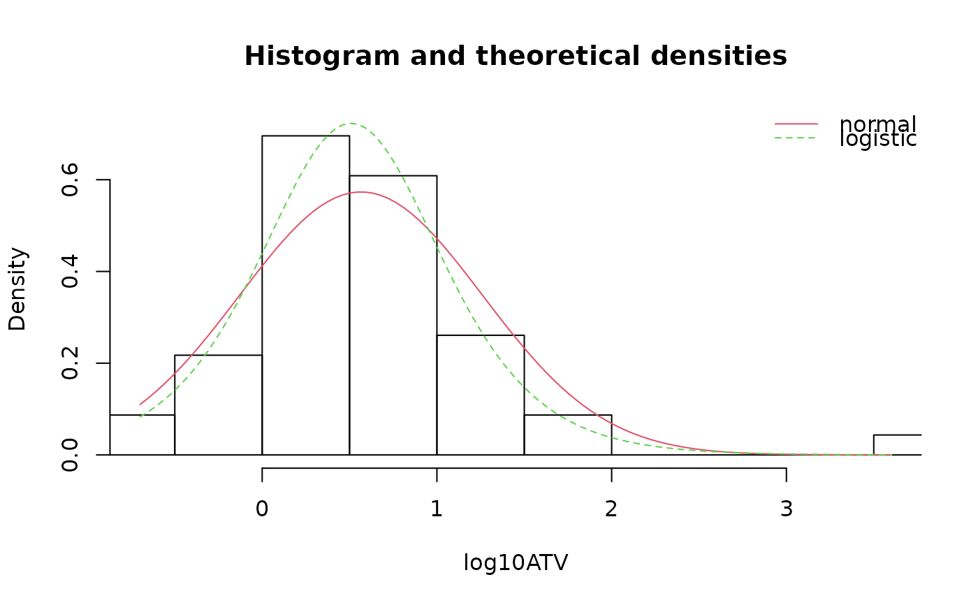
denscomp(list(fln,fll),legendtext=c("normal","logistic"),
xlab="log10ATV")


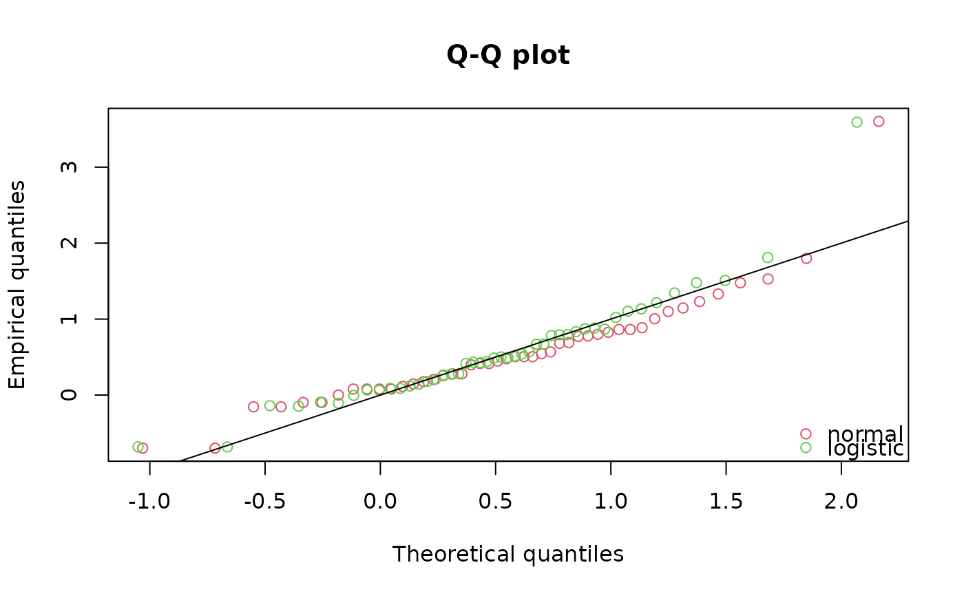
qqcomp(list(fln,fll),legendtext=c("normal","logistic"))

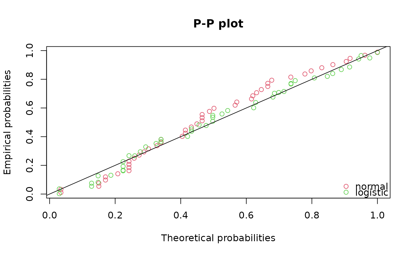
ppcomp(list(fln,fll),legendtext=c("normal","logistic"))


gofstat(list(fln,fll), fitnames = c("lognormal", "loglogistic"))
#> Goodness-of-fit statistics
#>                              lognormal loglogistic
#> Kolmogorov-Smirnov statistic 0.1267649  0.08457997
#> Cramer-von Mises statistic   0.1555576  0.04058514
#> Anderson-Darling statistic   1.0408045  0.37407465
#> 
#> Goodness-of-fit criteria
#>                                lognormal loglogistic
#> Akaike's Information Criterion  101.1751    92.63650
#> Bayesian Information Criterion  104.8324    96.29378

# (4) estimation of the 5 percent quantile value of 
# logistic fitted distribution (5 percent hazardous concentration  : HC5)
# with its two-sided 95 percent confidence interval calculated by 
# parametric bootstrap 
# with a small number of iterations to satisfy CRAN running times constraint.
# For practical applications, we recommend to use at least niter=501 or niter=1001.
#
# in log10(ATV)
bll <- bootdist(fll,niter=51)
HC5ll <- quantile(bll,probs = 0.05)
# in ATV
10^(HC5ll$quantiles)
#>            p=0.05
#> estimate 0.309253
10^(HC5ll$quantCI)
#>           p=0.05
#> 2.5 %  0.1891451
#> 97.5 % 0.5457214

# (5) estimation of the 5 percent quantile value of 
# the fitted logistic distribution (5 percent hazardous concentration  : HC5)
# with its one-sided 95 percent confidence interval (type "greater")
# calculated by 
# nonparametric bootstrap 
# with a small number of iterations to satisfy CRAN running times constraint.
# For practical applications, we recommend to use at least niter=501 or niter=1001.
# 
# in log10(ATV)
bllnonpar <- bootdist(fll,niter=51,bootmethod = "nonparam")
HC5llgreater <- quantile(bllnonpar,probs = 0.05, CI.type="greater")
# in ATV
10^(HC5llgreater$quantiles)
#>            p=0.05
#> estimate 0.309253
10^(HC5llgreater$quantCI)
#>        p=0.05
#> 5 % 0.1860103

# (6) fit of a logistic distribution 
# by minimizing the modified Anderson-Darling AD2L distance
# cf. ?mgedist for definition of this distance
#

fllAD2L <- fitdist(log10ATV,"logis",method="mge",gof="AD2L")
summary(fllAD2L)
#> Fitting of the distribution ' logis ' by maximum goodness-of-fit 
#> Parameters : 
#>           estimate
#> location 0.4965288
#> scale    0.3013154
#> Loglikelihood:  -44.96884   AIC:  93.93767   BIC:  97.59496 
plot(fllAD2L)