Species-Sensitivity Distribution (SSD) for Fluazinam

48-hour acute toxicity values (EC50 values) for exposure of macroinvertebrates and zooplancton to fluazinam.

Usage

data(fluazinam)

Format

fluazinam is a data frame with 2 columns named left and right, describing each observed EC50 value (in micrograms per liter) as an interval. The left column contains either NA for left censored observations, the left bound of the interval for interval censored observations, or the observed value for non-censored observations. The right column contains either NA for right censored observations, the right bound of the interval for interval censored observations, or the observed value for noncensored observations.

Source

Hose, G.C., Van den Brink, P.J. 2004. The species sensitivity distribution approach compared to a microcosm study: A case study with the fungicide fluazinam. Ecotoxicology and Environmental Safety, 73, 109-122.

Examples

# (1) load of data
#
data(fluazinam)

# (2) plot of data using Turnbull cdf plot
#
log10EC50 <- log10(fluazinam)
plotdistcens(log10EC50)


# (3) fit of a lognormal and a logistic distribution to data
# (classical distributions used for species sensitivity 
# distributions, SSD, in ecotoxicology)
# and visual comparison of the fits using Turnbull cdf plot 
#
fln <- fitdistcens(log10EC50, "norm")
summary(fln)
#> Fitting of the distribution ' norm ' By maximum likelihood on censored data 
#> Parameters
#>      estimate Std. Error
#> mean 2.161449  1.2060732
#> sd   1.167290  0.9842019
#> Loglikelihood:  -20.41212   AIC:  44.82424   BIC:  46.10235 
#> Correlation matrix:
#>           mean        sd
#> mean 1.0000000 0.1350237
#> sd   0.1350237 1.0000000
#> 

fll <- fitdistcens(log10EC50, "logis")
summary(fll)
#> Fitting of the distribution ' logis ' By maximum likelihood on censored data 
#> Parameters
#>           estimate Std. Error
#> location 2.1518291  1.2058724
#> scale    0.6910423  0.6530058
#> Loglikelihood:  -20.55391   AIC:  45.10781   BIC:  46.38593 
#> Correlation matrix:
#>            location      scale
#> location 1.00000000 0.05097494
#> scale    0.05097494 1.00000000
#> 

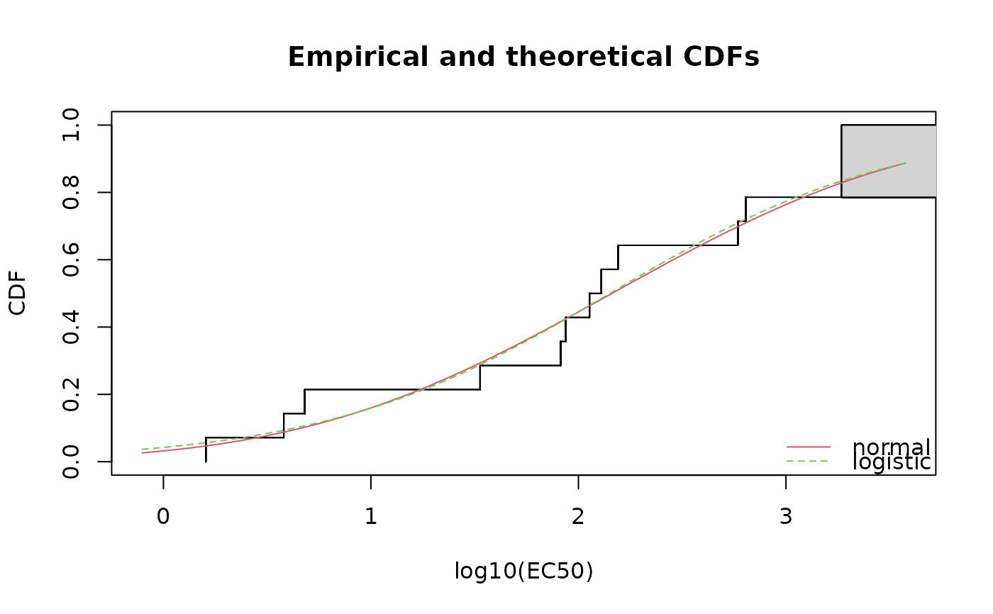
cdfcompcens(list(fln,fll), legendtext = c("normal", "logistic"), 
  xlab = "log10(EC50)")


# (4) estimation of the 5 percent quantile value of 
# the normal fitted distribution (5 percent hazardous concentration  : HC5)
# with its two-sided 95 percent confidence interval calculated by 
# non parametric bootstrap
# with a small number of iterations to satisfy CRAN running times constraint.
# For practical applications, we recommend to use at least niter=501 or niter=1001.
#
# in log10(EC50)
bln <- bootdistcens(fln, niter = 101)
HC5ln <- quantile(bln, probs = 0.05)
# in EC50
10^(HC5ln$quantiles)
#>            p=0.05
#> estimate 1.743522
10^(HC5ln$quantCI)
#>            p=0.05
#> 2.5 %   0.3021309
#> 97.5 % 13.5760675

# (5) estimation of the HC5 value
# with its one-sided 95 percent confidence interval (type "greater")
#
# in log10(EC50)
HC5lnb <- quantile(bln, probs = 0.05, CI.type = "greater")

# in LC50
10^(HC5lnb$quantiles)
#>            p=0.05
#> estimate 1.743522
10^(HC5lnb$quantCI)
#>        p=0.05
#> 5 % 0.4182488