(Log)likelihood surfaces or (log)likelihood curves

llsurface plots the likelihood surface for distributions with two or more parameters, llcurve plots the likelihood curve for distributions with one or more parameters.

Usage

llsurface(data, distr, plot.arg, min.arg, max.arg,   lseq = 50, fix.arg = NULL,  
    loglik = TRUE, back.col = TRUE, nlev = 10, pal.col = terrain.colors(100), 
    weights = NULL, ...)    

llcurve(data, distr, plot.arg, min.arg, max.arg,   lseq = 50, fix.arg = NULL,  
    loglik = TRUE, weights = NULL, ...)

Arguments

data: A numeric vector for non censored data or a dataframe of two columns respectively named left and right, describing each observed value as an interval for censored data. In that case the left column contains either NA for left censored observations, the left bound of the interval for interval censored observations, or the observed value for non-censored observations. The right column contains either NA for right censored observations, the right bound of the interval for interval censored observations, or the observed value for non-censored observations.
distr: A character string "name" naming a distribution for which the corresponding density function dname and the corresponding distribution function pname must be classically defined.
plot.arg: a two-element vector with the names of the two parameters that will vary for llsurface, only one element for llcurve.
min.arg: a two-element vector with lower plotting bounds for llsurface, only one element for llcurve.
max.arg: a two-element vector with upper plotting bounds for llsurface, only one element for llcurve.
lseq: length of sequences of parameters.
fix.arg: a named list with fixed value of other parameters.
loglik: a logical to plot log-likelihood or likelihood function.
back.col: logical (for llsurface only). Contours are plotted with a background gradient of colors if TRUE.
nlev: number of contour levels to plot (for llsurface only).
pal.col: Palette of colors. Colors to be used as back (for llsurface only).
weights: an optional vector of weights to be used in the fitting process. Should be NULL or a numeric vector with strictly positive values (classically the number of occurences of each observation).
...: Further graphical arguments passed to graphical functions.

Details

These two function are not intended to be called directly but is internally called in llplot.

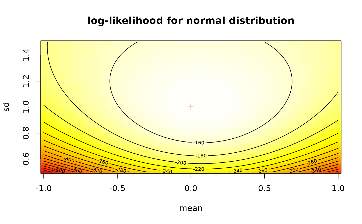
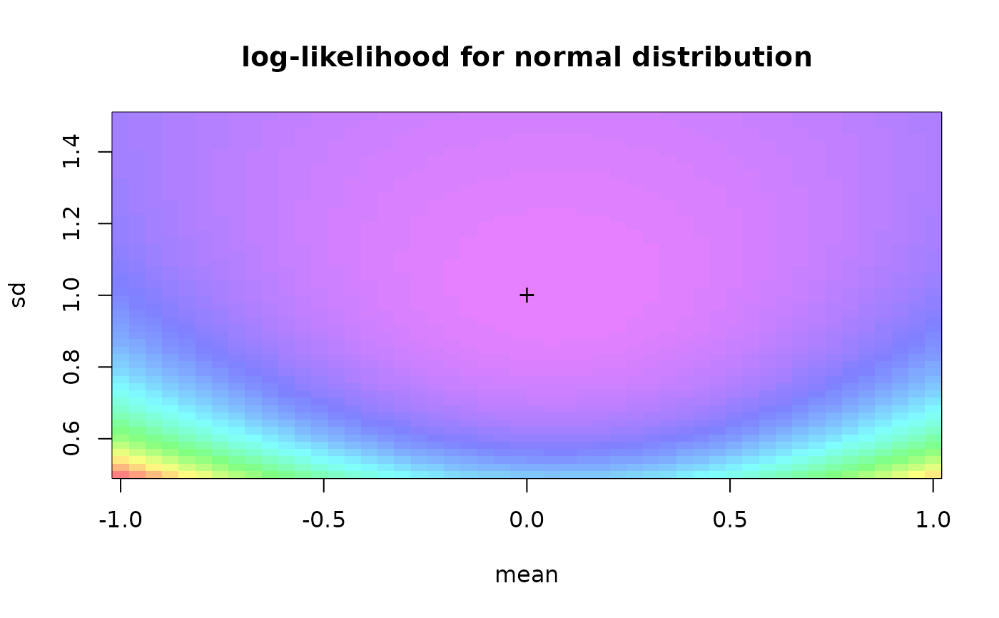
llsurface plots the likelihood surface for distributions with two varying parameters and other parameters fixed. When back.col, image (2D-plot) is used. When nlev > 0, contour (2D-plot) is used to add nlev contours.

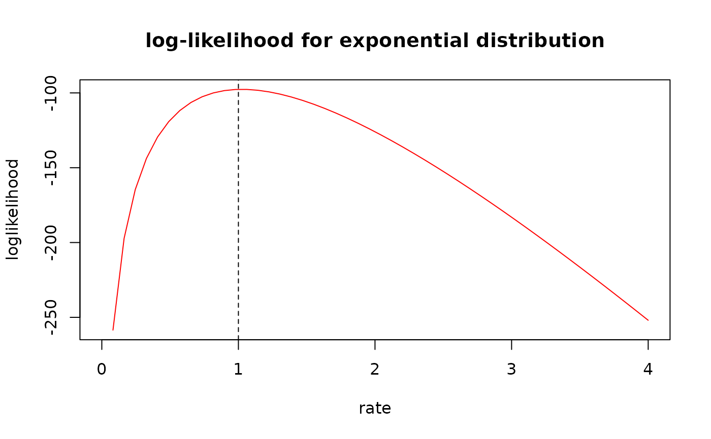
llcurve plots the likelihood curve for distributions with one varying parameter and other parameters fixed.

References

Delignette-Muller ML and Dutang C (2015), fitdistrplus: An R Package for Fitting Distributions. Journal of Statistical Software, 64(4), 1-34, doi:10.18637/jss.v064.i04 .

Author

Marie-Laure Delignette-Muller and Christophe Dutang.

Examples

# (1) loglikelihood or likelihood curve
#

n <- 100
set.seed(1234)
x <- rexp(n)

llcurve(data = x, distr = "exp", plot.arg =  "rate", min.arg = 0, max.arg = 4)


llcurve(data = x, distr = "exp", plot.arg =  "rate", min.arg = 0, max.arg = 4, 
loglik = FALSE)


llcurve(data = x, distr = "exp", plot.arg =  "rate", min.arg = 0, max.arg = 4, 
  main = "log-likelihood for exponential distribution", col = "red")
abline(v = 1, lty = 2)



# (2) loglikelihood surface
# 

x <- rnorm(n, 0, 1)

llsurface(data =x, distr="norm", plot.arg=c("mean", "sd"), 
          min.arg=c(-1, 0.5), max.arg=c(1, 3/2), back.col = FALSE,
          main="log-likelihood for normal distribution")

llsurface(data =x, distr="norm", plot.arg=c("mean", "sd"), 
          min.arg=c(-1, 0.5), max.arg=c(1, 3/2), 
          main="log-likelihood for normal distribution", 
          nlev = 20, pal.col = heat.colors(100),)
points(0, 1, pch="+", col="red")

llsurface(data =x, distr="norm", plot.arg=c("mean", "sd"), 
          min.arg=c(-1, 0.5), max.arg=c(1, 3/2), 
          main="log-likelihood for normal distribution", 
          nlev = 0, back.col = TRUE, pal.col = rainbow(100, s = 0.5, end = 0.8))
points(0, 1, pch="+", col="black")