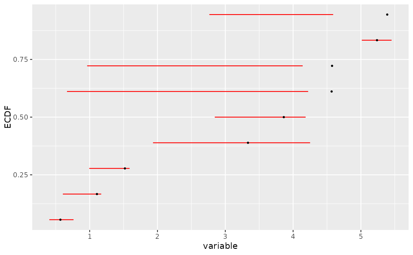
ECDF plot of a variable with given confidence intervals on this variable
ecdfplotwithCI.RdProvides an ECDF plot of a variable, with x-error bars for given confidence intervals on this variable, possibly partitioned by groups. In the context of this package this function is intended to be used with the BMD as the variable and with groups defined by the user from functional annotation.
Usage
ecdfplotwithCI(variable, CI.lower, CI.upper, by, CI.col = "blue",
CI.alpha = 1, add.point = TRUE, point.size = 1, point.type = 16)
Arguments
- variable
A numeric vector of the variable to plot. In the context of the package this variable may be a BMD.
- CI.lower
A corresponding numeric vector (same length) with the lower bounds of the confidence intervals.
- CI.upper
A corresponding numeric vector (same length) with the upper bounds of the confidence intervals.
- by
A factor of the same length for split of the plot by this factor (no split if omitted). In the context of this package this factor may code for groups defined by the user from functional annotation.
- CI.col
The color to draw the confidence intervals (unique color) of a factor coding for the color.
- CI.alpha
Optional transparency of the lines used to draw the confidence intervals.
- add.point
If
TRUEpoints are added to confidence intervals.- point.size
Size of the added points in case
add.pointisTRUE.- point.type
Shape of the added points in case
add.pointisTRUEdefined as an integer coding for a unique common shape or as a factor coding for the shape.
See also
See plot.bmdboot.
Examples
# (1) a toy example (a very small subsample of a microarray data set)
#
datafilename <- system.file("extdata", "transcripto_very_small_sample.txt",
package="DRomics")
o <- microarraydata(datafilename, check = TRUE, norm.method = "cyclicloess")
#> Just wait, the normalization using cyclicloess may take a few minutes.
s_quad <- itemselect(o, select.method = "quadratic", FDR = 0.001)
#> Removing intercept from test coefficients
f <- drcfit(s_quad, progressbar = TRUE)
#> The fitting may be long if the number of selected items is high.
#>
|
| | 0%
|
|======= | 10%
|
|============== | 20%
|
|===================== | 30%
|
|============================ | 40%
|
|=================================== | 50%
|
|========================================== | 60%
|
|================================================= | 70%
|
|======================================================== | 80%
|
|=============================================================== | 90%
|
|======================================================================| 100%
r <- bmdcalc(f)
set.seed(1) # to get reproducible results with a so small number of iterations
b <- bmdboot(r, niter = 5) # with a non reasonable value for niter
#> Warning:
#> A small number of iterations (less than 1000) may not be sufficient to
#> ensure a good quality of bootstrap confidence intervals.
#> The bootstrap may be long if the number of items and the number of
#> bootstrap iterations is high.
#>
|
| | 0%
|
|======= | 10%
|
|============== | 20%
|
|===================== | 30%
|
|============================ | 40%
|
|========================================== | 60%
|
|================================================= | 70%
|
|======================================================== | 80%
|
|=============================================================== | 90%
|
|======================================================================| 100%
# !!!! TO GET CORRECT RESULTS
# !!!! niter SHOULD BE FIXED FAR LARGER , e.g. to 1000
# !!!! but the run will be longer
# manual ecdf plot of the bootstrap results as an ecdf distribution
# on BMD, plot that could also be obtained with plot(b)
# in this simple case
#
a <- b$res[is.finite(b$res$BMD.zSD.upper), ]
ecdfplotwithCI(variable = a$BMD.zSD, CI.lower = a$BMD.zSD.lower,
CI.upper = a$BMD.zSD.upper, CI.col = "red")
#> `height` was translated to `width`.
 # \donttest{
# (2) An example from data published by Larras et al. 2020
# in Journal of Hazardous Materials
# https://doi.org/10.1016/j.jhazmat.2020.122727
# This function can also be used to go deeper in the exploration of the biological
# meaning of the responses. Here is an example linking the DRomics outputs
# with the functional annotation of the responding metabolites of the microalgae
# Scenedesmus vacuolatus to the biocide triclosan.
# This extra step uses a dataframe previously built by the user which links the items
# to the biological information of interest (e.g. KEGG pathways).
# importation of a dataframe with metabolomic results
# (output $res of bmdcalc() or bmdboot() functions)
resfilename <- system.file("extdata", "triclosanSVmetabres.txt", package="DRomics")
res <- read.table(resfilename, header = TRUE, stringsAsFactors = TRUE)
str(res)
#> 'data.frame': 31 obs. of 27 variables:
#> $ id : Factor w/ 31 levels "NAP47_51","NAP_2",..: 2 3 4 5 6 7 8 9 10 11 ...
#> $ irow : int 2 21 28 34 38 47 49 51 53 67 ...
#> $ adjpvalue : num 6.23e-05 1.11e-05 1.03e-05 1.89e-03 4.16e-03 ...
#> $ model : Factor w/ 4 levels "Gauss-probit",..: 2 3 3 2 2 4 2 2 3 3 ...
#> $ nbpar : int 3 2 2 3 3 5 3 3 2 2 ...
#> $ b : num 0.4598 -0.0595 -0.0451 0.6011 0.6721 ...
#> $ c : num NA NA NA NA NA ...
#> $ d : num 5.94 5.39 7.86 6.86 6.21 ...
#> $ e : num -1.648 NA NA -0.321 -0.323 ...
#> $ f : num NA NA NA NA NA ...
#> $ SDres : num 0.126 0.0793 0.052 0.2338 0.2897 ...
#> $ typology : Factor w/ 10 levels "E.dec.concave",..: 2 7 7 2 2 9 2 2 7 7 ...
#> $ trend : Factor w/ 4 levels "U","bell","dec",..: 3 3 3 3 3 1 3 3 3 3 ...
#> $ y0 : num 5.94 5.39 7.86 6.86 6.21 ...
#> $ yrange : num 0.456 0.461 0.35 0.601 0.672 ...
#> $ maxychange : num 0.456 0.461 0.35 0.601 0.672 ...
#> $ xextrem : num NA NA NA NA NA ...
#> $ yextrem : num NA NA NA NA NA ...
#> $ BMD.zSD : num 0.528 1.333 1.154 0.158 0.182 ...
#> $ BMR.zSD : num 5.82 5.31 7.81 6.62 5.92 ...
#> $ BMD.xfold : num NA NA NA NA 0.832 ...
#> $ BMR.xfold : num 5.35 4.85 7.07 6.17 5.59 ...
#> $ BMD.zSD.lower : num 0.2001 0.8534 0.7519 0.0554 0.081 ...
#> $ BMD.zSD.upper : num 1.11 1.746 1.465 0.68 0.794 ...
#> $ BMD.xfold.lower : num Inf 7.611 Inf 0.561 0.329 ...
#> $ BMD.xfold.upper : num Inf Inf Inf Inf Inf ...
#> $ nboot.successful: int 957 1000 1000 648 620 872 909 565 1000 1000 ...
# importation of a dataframe with annotation of each item
# identified in the previous file (this dataframe must be previously built by the user)
# each item may have more than one annotation (-> more than one line)
annotfilename <- system.file("extdata", "triclosanSVmetabannot.txt", package="DRomics")
annot <- read.table(annotfilename, header = TRUE, stringsAsFactors = TRUE)
str(annot)
#> 'data.frame': 84 obs. of 2 variables:
#> $ metab.code: Factor w/ 31 levels "NAP47_51","NAP_2",..: 2 3 4 4 4 4 5 6 7 8 ...
#> $ path_class: Factor w/ 9 levels "Amino acid metabolism",..: 5 3 3 2 6 8 5 5 5 5 ...
# Merging of both previous dataframes
# in order to obtain an extenderes dataframe
# bootstrap results and annotation
annotres <- merge(x = res, y = annot, by.x = "id", by.y = "metab.code")
head(annotres)
#> id irow adjpvalue model nbpar b c d
#> 1 NAP47_51 46 7.158246e-04 linear 2 -0.05600559 NA 7.343571
#> 2 NAP_2 2 6.232579e-05 exponential 3 0.45981242 NA 5.941896
#> 3 NAP_23 21 1.106958e-05 linear 2 -0.05946618 NA 5.387252
#> 4 NAP_30 28 1.028343e-05 linear 2 -0.04507832 NA 7.859109
#> 5 NAP_30 28 1.028343e-05 linear 2 -0.04507832 NA 7.859109
#> 6 NAP_30 28 1.028343e-05 linear 2 -0.04507832 NA 7.859109
#> e f SDres typology trend y0 yrange maxychange
#> 1 NA NA 0.12454183 L.dec dec 7.343571 0.4346034 0.4346034
#> 2 -1.647958 NA 0.12604568 E.dec.convex dec 5.941896 0.4556672 0.4556672
#> 3 NA NA 0.07929266 L.dec dec 5.387252 0.4614576 0.4614576
#> 4 NA NA 0.05203245 L.dec dec 7.859109 0.3498078 0.3498078
#> 5 NA NA 0.05203245 L.dec dec 7.859109 0.3498078 0.3498078
#> 6 NA NA 0.05203245 L.dec dec 7.859109 0.3498078 0.3498078
#> xextrem yextrem BMD.zSD BMR.zSD BMD.xfold BMR.xfold BMD.zSD.lower
#> 1 NA NA 2.2237393 7.219029 NA 6.609214 0.9785095
#> 2 NA NA 0.5279668 5.815850 NA 5.347706 0.2000881
#> 3 NA NA 1.3334076 5.307960 NA 4.848527 0.8533711
#> 4 NA NA 1.1542677 7.807077 NA 7.073198 0.7518588
#> 5 NA NA 1.1542677 7.807077 NA 7.073198 0.7518588
#> 6 NA NA 1.1542677 7.807077 NA 7.073198 0.7518588
#> BMD.zSD.upper BMD.xfold.lower BMD.xfold.upper nboot.successful
#> 1 4.068699 Inf Inf 1000
#> 2 1.109559 Inf Inf 957
#> 3 1.746010 7.610936 Inf 1000
#> 4 1.464998 Inf Inf 1000
#> 5 1.464998 Inf Inf 1000
#> 6 1.464998 Inf Inf 1000
#> path_class
#> 1 Lipid metabolism
#> 2 Lipid metabolism
#> 3 Carbohydrate metabolism
#> 4 Carbohydrate metabolism
#> 5 Biosynthesis of other secondary metabolites
#> 6 Membrane transport
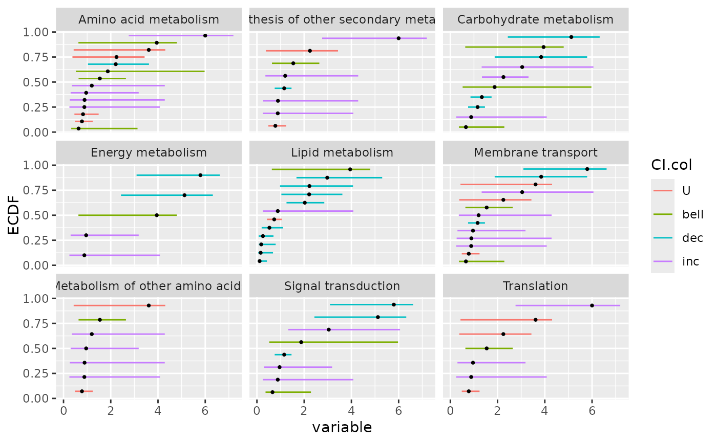
### an ECDFplot with confidence intervals by pathway
# with color coding for dose-response trend
ecdfplotwithCI(variable = annotres$BMD.zSD,
CI.lower = annotres$BMD.zSD.lower,
CI.upper = annotres$BMD.zSD.upper,
by = annotres$path_class,
CI.col = annotres$trend)
#> `height` was translated to `width`.
 # (3) an example on a microarray data set (a subsample of a greater data set)
#
datafilename <- system.file("extdata", "transcripto_sample.txt", package="DRomics")
(o <- microarraydata(datafilename, check = TRUE, norm.method = "cyclicloess"))
#> Just wait, the normalization using cyclicloess may take a few minutes.
#> Elements of the experimental design in order to check the coding of the data:
#> Tested doses and number of replicates for each dose:
#>
#> 0 0.69 1.223 2.148 3.774 6.631
#> 5 5 5 5 5 5
#> Number of items: 1000
#> Identifiers of the first 20 items:
#> [1] "1" "2" "3" "4" "5.1" "5.2" "6.1" "6.2" "7.1" "7.2"
#> [11] "8.1" "8.2" "9.1" "9.2" "10.1" "10.2" "11.1" "11.2" "12.1" "12.2"
#> Data were normalized between arrays using the following method: cyclicloess
(s_quad <- itemselect(o, select.method = "quadratic", FDR = 0.001))
#> Removing intercept from test coefficients
#> Number of selected items using a quadratic trend test with an FDR of 0.001: 78
#> Identifiers of the first 20 most responsive items:
#> [1] "384.2" "383.1" "383.2" "384.1" "301.1" "363.1" "300.2" "364.2" "364.1"
#> [10] "363.2" "301.2" "300.1" "351.1" "350.2" "239.1" "240.1" "240.2" "370"
#> [19] "15" "350.1"
(f <- drcfit(s_quad, progressbar = TRUE))
#> The fitting may be long if the number of selected items is high.
#>
|
| | 0%
|
|= | 1%
|
|== | 3%
|
|=== | 4%
|
|==== | 5%
|
|==== | 6%
|
|===== | 8%
|
|====== | 9%
|
|======= | 10%
|
|======== | 12%
|
|========= | 13%
|
|========== | 14%
|
|=========== | 15%
|
|============ | 17%
|
|============= | 18%
|
|============= | 19%
|
|============== | 21%
|
|=============== | 22%
|
|================ | 23%
|
|================= | 24%
|
|================== | 26%
|
|=================== | 27%
|
|==================== | 28%
|
|===================== | 29%
|
|====================== | 31%
|
|====================== | 32%
|
|======================= | 33%
|
|======================== | 35%
|
|========================= | 36%
|
|========================== | 37%
|
|=========================== | 38%
|
|============================ | 40%
|
|============================= | 41%
|
|============================== | 42%
|
|=============================== | 44%
|
|=============================== | 45%
|
|================================ | 46%
|
|================================= | 47%
|
|================================== | 49%
|
|=================================== | 50%
|
|==================================== | 51%
|
|===================================== | 53%
|
|====================================== | 54%
|
|======================================= | 55%
|
|======================================= | 56%
|
|======================================== | 58%
|
|========================================= | 59%
|
|========================================== | 60%
|
|=========================================== | 62%
|
|============================================ | 63%
|
|============================================= | 64%
|
|============================================== | 65%
|
|=============================================== | 67%
|
|================================================ | 68%
|
|================================================ | 69%
|
|================================================= | 71%
|
|================================================== | 72%
|
|=================================================== | 73%
|
|==================================================== | 74%
|
|===================================================== | 76%
|
|====================================================== | 77%
|
|======================================================= | 78%
|
|======================================================== | 79%
|
|========================================================= | 81%
|
|========================================================= | 82%
|
|========================================================== | 83%
|
|=========================================================== | 85%
|
|============================================================ | 86%
|
|============================================================= | 87%
|
|============================================================== | 88%
|
|=============================================================== | 90%
|
|================================================================ | 91%
|
|================================================================= | 92%
|
|================================================================== | 94%
|
|================================================================== | 95%
|
|=================================================================== | 96%
|
|==================================================================== | 97%
|
|===================================================================== | 99%
|
|======================================================================| 100%
#> Results of the fitting using the AICc to select the best fit model
#> 11 dose-response curves out of 78 previously selected were removed
#> because no model could be fitted reliably.
#> Distribution of the chosen models among the 67 fitted dose-response curves:
#>
#> Hill linear exponential Gauss-probit
#> 0 11 30 23
#> log-Gauss-probit
#> 3
#> Distribution of the trends (curve shapes) among the 67 fitted dose-response curves:
#>
#> U bell dec inc
#> 6 20 22 19
(r <- bmdcalc(f))
#> 1 BMD-xfold values and 0 BMD-zSD values are not defined (coded NaN as
#> the BMR stands outside the range of response values defined by the model).
#> 28 BMD-xfold values and 0 BMD-zSD values could not be calculated (coded
#> NA as the BMR stands within the range of response values defined by the
#> model but outside the range of tested doses).
(b <- bmdboot(r, niter = 100)) # niter to put at 1000 for a better precision
#> Warning:
#> A small number of iterations (less than 1000) may not be sufficient to
#> ensure a good quality of bootstrap confidence intervals.
#> The bootstrap may be long if the number of items and the number of
#> bootstrap iterations is high.
#>
|
| | 0%
|
|= | 1%
|
|== | 3%
|
|=== | 4%
|
|==== | 6%
|
|===== | 7%
|
|====== | 9%
|
|======= | 10%
|
|======== | 12%
|
|========= | 13%
|
|========== | 15%
|
|=========== | 16%
|
|============= | 18%
|
|============== | 19%
|
|=============== | 21%
|
|================ | 22%
|
|================= | 24%
|
|================== | 25%
|
|=================== | 27%
|
|==================== | 28%
|
|===================== | 30%
|
|====================== | 31%
|
|======================= | 33%
|
|======================== | 34%
|
|========================= | 36%
|
|========================== | 37%
|
|=========================== | 39%
|
|============================ | 40%
|
|============================= | 42%
|
|============================== | 43%
|
|=============================== | 45%
|
|================================ | 46%
|
|================================= | 48%
|
|================================== | 49%
|
|==================================== | 51%
|
|===================================== | 52%
|
|====================================== | 54%
|
|======================================= | 55%
|
|======================================== | 57%
|
|========================================= | 58%
|
|=========================================== | 61%
|
|============================================ | 63%
|
|============================================= | 64%
|
|============================================== | 66%
|
|=============================================== | 67%
|
|================================================ | 69%
|
|================================================= | 70%
|
|================================================== | 72%
|
|=================================================== | 73%
|
|==================================================== | 75%
|
|===================================================== | 76%
|
|====================================================== | 78%
|
|========================================================= | 82%
|
|=========================================================== | 84%
|
|============================================================ | 85%
|
|============================================================= | 87%
|
|============================================================== | 88%
|
|=============================================================== | 90%
|
|================================================================ | 91%
|
|================================================================= | 93%
|
|=================================================================== | 96%
|
|==================================================================== | 97%
|
|===================================================================== | 99%
|
|======================================================================| 100%
#> Bootstrap confidence interval computation failed on 4 items among 67
#> due to lack of convergence of the model fit for a fraction of the
#> bootstrapped samples greater than 0.5.
#> For 0 BMD.zSD values and 35 BMD.xfold values among 67 at least one
#> bound of the 95 percent confidence interval could not be computed due
#> to some bootstrapped BMD values not reachable due to model asymptotes
#> or reached outside the range of tested doses (bounds coded Inf)).
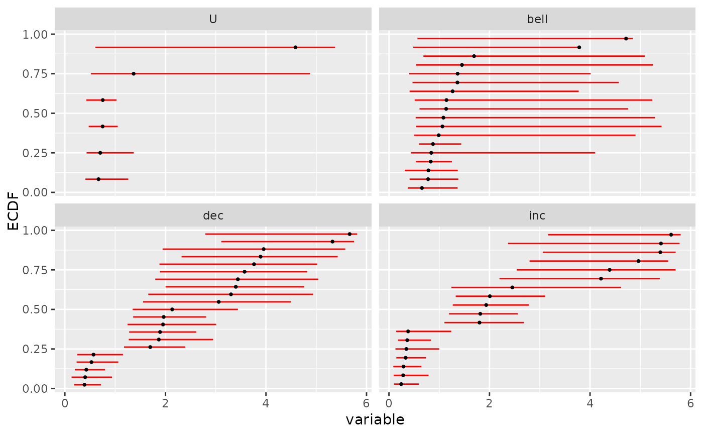
# (3.a)
# manual ecdf plot of the bootstrap results as an ecdf distribution
# on BMD for each trend
# plot that could also be obtained with plot(b, by = "trend")
# in this simple case
#
a <- b$res[is.finite(b$res$BMD.zSD.upper), ]
ecdfplotwithCI(variable = a$BMD.zSD, CI.lower = a$BMD.zSD.lower,
CI.upper = a$BMD.zSD.upper, by = a$trend, CI.col = "red")
#> `height` was translated to `width`.
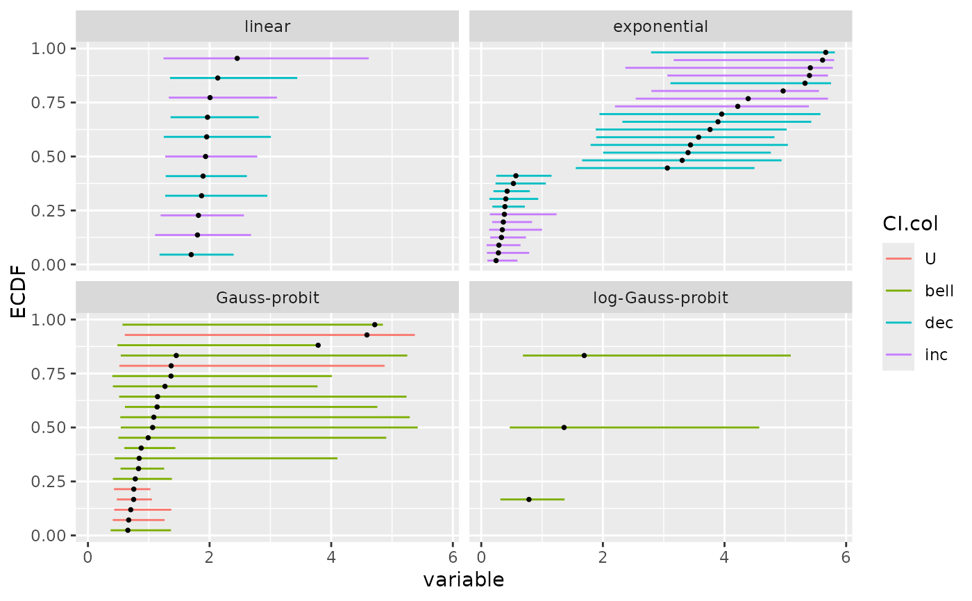
 # (3.b)
# ecdf plot of the bootstrap results as an ecdf distribution
# on BMD for each model
# with the color of the confidence intervals coding for the trend
#
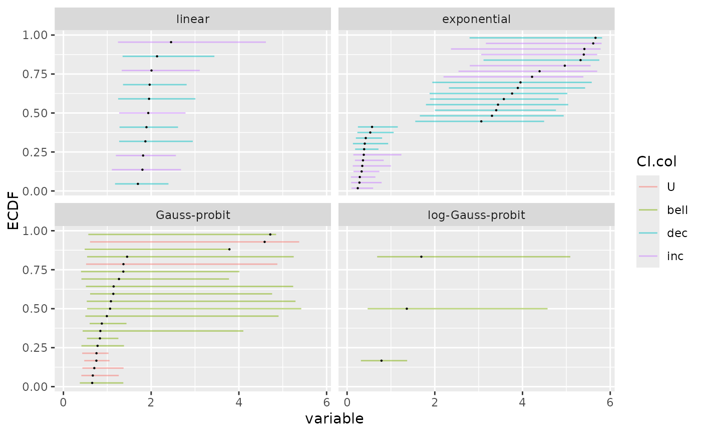
ecdfplotwithCI(variable = a$BMD.zSD, CI.lower = a$BMD.zSD.lower,
CI.upper = a$BMD.zSD.upper, by = a$model, CI.col = a$trend)
#> `height` was translated to `width`.
 # changing the size of the points and the transparency of CI lines
ecdfplotwithCI(variable = a$BMD.zSD, CI.lower = a$BMD.zSD.lower,
CI.upper = a$BMD.zSD.upper, by = a$model, CI.col = a$trend,
CI.alpha = 0.5, point.size = 0.5)
#> `height` was translated to `width`.
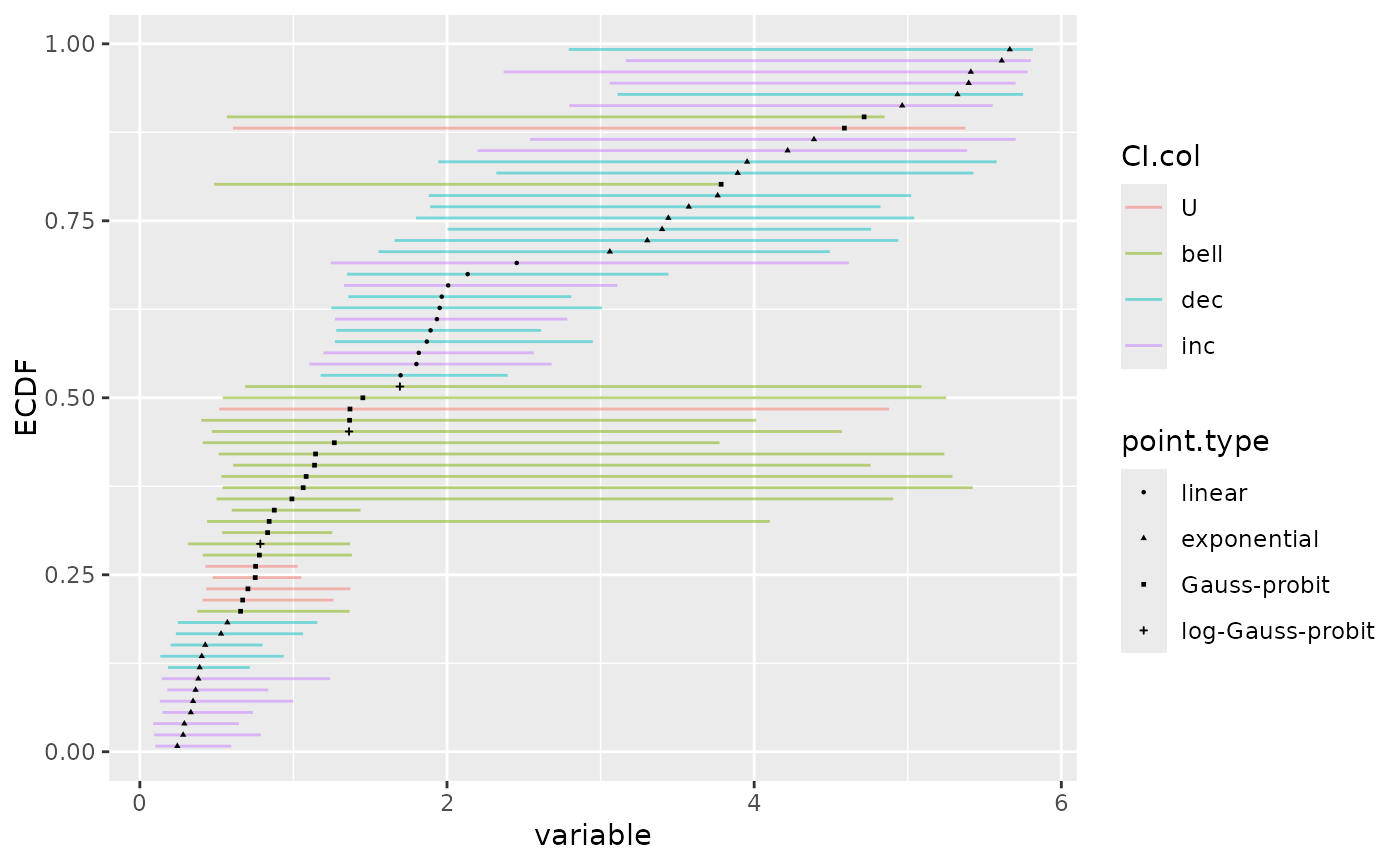
 # with the model coding for the type of points
ecdfplotwithCI(variable = a$BMD.zSD, CI.lower = a$BMD.zSD.lower,
CI.upper = a$BMD.zSD.upper, CI.col = a$trend,
CI.alpha = 0.5, point.size = 0.5, point.type = a$model)
#> `height` was translated to `width`.
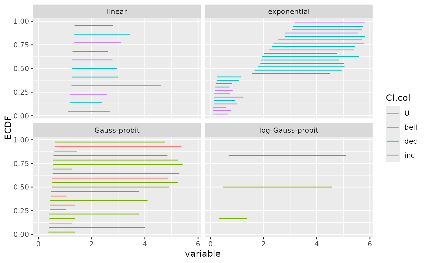
 # (3.c)
# ecdf plot of the bootstrap results as an ecdf distribution on
# on BMD_L (lower value of the confidence interval) for each trend
#
ecdfplotwithCI(variable = a$BMD.zSD.lower, CI.lower = a$BMD.zSD.lower,
CI.upper = a$BMD.zSD.upper, by = a$model, CI.col = a$trend,
add.point = FALSE)
#> `height` was translated to `width`.
 # }
# }