Computation of confidence interval on benchmark doses by bootstrap
bmdboot.RdComputes 95 percent confidence intervals on x-fold and z-SD benchmark doses by bootstrap.
Usage
bmdboot(r, items = r$res$id, niter = 1000,
                    conf.level = 0.95,
                    tol = 0.5, progressbar = TRUE,
                    parallel = c("no", "snow", "multicore"), ncpus)

# S3 method for class 'bmdboot'
print(x, ...)

# S3 method for class 'bmdboot'
plot(x, BMDtype = c("zSD", "xfold"), remove.infinite = TRUE,
                   by = c("none", "trend", "model", "typology"),
                   CI.col = "blue", BMD_log_transfo = TRUE,  ...)
Arguments
- r
An object of class
"bmdcalc"returned by the functionbmdcalc.- items
A character vector specifying the identifiers of the items for which you want the computation of confidence intervals. If omitted the computation is done for all the items.
- niter
The number of samples drawn by bootstrap.
- conf.level
Confidence level of the intervals.
- tol
The tolerance in term of proportion of bootstrap samples on which the fit of the model is successful (if this proportion is below the tolerance, NA values are given for the limits of the confidence interval.
- progressbar
If
TRUEa progress bar is used to follow the bootstrap process.- parallel
The type of parallel operation to be used,
"snow"or"multicore"(the second one not being available on Windows), or"no"if no parallel operation.- ncpus
Number of processes to be used in parallel operation : typically one would fix it to the number of available CPUs.
- x
An object of class
"bmdboot".- BMDtype
The type of BMD to plot,
"zSD"(default choice) or"xfold".- remove.infinite
If TRUE the confidence intervals with non finite upper bound are not plotted.
- by
If not at
"none"the plot is split by the indicated factor ("trend","model"or"typology").- CI.col
The color to draw the confidence intervals.
- BMD_log_transfo
If TRUE, default option, a log transformation of the BMD is used in the plot.
- ...
Further arguments passed to graphical or print functions.
Details
Non-parametric bootstrapping is used, where mean centered residuals are bootstrapped.
For each item, bootstrapped parameter estimates are obtained by fitting the model on each of the resampled data sets. If the fitting procedure fails to converge in more than tol*100% of the cases, NA values are given for the confidence interval. Otherwise, bootstraped
BMD are computed from bootstrapped parameter estimates using the same method as
in bmdcalc.
Confidence intervals on BMD are then
computed using percentiles of the bootstrapped BMDs.
For example 95 percent confidence intervals are
computed using 2.5 and 97.5 percentiles of the bootstrapped BMDs.
In cases where the bootstrapped BMD cannot be estimated as
not reached at the highest tested dose or not reachable due to model asymptotes,
it was given an infinite value Inf, so as to enable the computation
of the lower limit of the BMD confidence interval if a sufficient number of bootstrapped BMD values were estimated
to finite values.
Value
bmdboot returns an object of class "bmdboot", a list with 3 components:
- res
a data frame reporting the results of the fit, BMD computation and bootstrap on each specified item sorted in the ascending order of the adjusted p-values. The different columns correspond to the identifier of each item (
id), the row number of this item in the initial data set (irow), the adjusted p-value of the selection step (adjpvalue), the name of the best fit model (model), the number of fitted parameters (nbpar), the values of the parametersb,c,d,eandf, (NAfor non used parameters), the residual standard deviation (SDres), the typology of the curve (typology, (16 class typology described in the help of thedrcfitfunction)), the rough trend of the curve (trend) defined with four classes (U, bell, increasing or decreasing shape), the theoretical y value at the control (y0), the theoretical y value at the maximal doseyatdosemax), the theoretical y range for x within the range of tested doses (yrange), the maximal absolute y change (up or down) from the control(maxychange) and for biphasic curves the x value at which their extremum is reached (xextrem) and the corresponding y value (yextrem), the BMD-zSD value (BMD.zSD) with the corresponding BMR-zSD value (reached or not,BMR.zSD) and the BMD-xfold value (BMD.xfold) with the corresponding BMR-xfold value (reached or not,BMR.xfold),BMD.zSD.lowerandBMD.zSD.upperthe lower and upper bounds of the confidence intervals of the BMD-zSD value,BMD.xfold.lowerandBMD.xfold.upperthe lower and upper bounds of the confidence intervals of the BMD-xfold value andnboot.successfulthe number of successful fits on bootstrapped samples for each item.- z
Value of z given in input to define the BMD-zSD.
- x
Value of x given in input as a percentage to define the BMD-xfold.
- tol
The tolerance given in input in term of tolerated proportion of failures of fit on bootstrapped samples.
- niter
The number of samples drawn by bootstrap (given in input).
See also
See bmdcalc for details about the computation of benchmark doses.
References
Huet S, Bouvier A, Poursat M-A, Jolivet E (2003) Statistical tools for nonlinear regression: a practical guide with S-PLUS and R examples. Springer, Berlin, Heidelberg, New York.
Examples
# (1) a toy example (a very small subsample of a microarray data set)
#
datafilename <- system.file("extdata", "transcripto_very_small_sample.txt",
package = "DRomics")
# to test the package on a small but not very small data set
# use the following commented line
# datafilename <- system.file("extdata", "transcripto_sample.txt", package = "DRomics")
o <- microarraydata(datafilename, check = TRUE, norm.method = "cyclicloess")
#> Just wait, the normalization using cyclicloess may take a few minutes.
s_quad <- itemselect(o, select.method = "quadratic", FDR = 0.001)
#> Removing intercept from test coefficients
f <- drcfit(s_quad, progressbar = TRUE)
#> The fitting may be long if the number of selected items is high.
#>
|
| | 0%
|
|======= | 10%
|
|============== | 20%
|
|===================== | 30%
|
|============================ | 40%
|
|=================================== | 50%
|
|========================================== | 60%
|
|================================================= | 70%
|
|======================================================== | 80%
|
|=============================================================== | 90%
|
|======================================================================| 100%
r <- bmdcalc(f)
set.seed(1234) # to get reproducible results with a so small number of iterations
(b <- bmdboot(r, niter = 5)) # with a non reasonable value for niter
#> Warning:
#> A small number of iterations (less than 1000) may not be sufficient to
#> ensure a good quality of bootstrap confidence intervals.
#> The bootstrap may be long if the number of items and the number of
#> bootstrap iterations is high.
#>
|
| | 0%
|
|======= | 10%
|
|============== | 20%
|
|===================== | 30%
|
|============================ | 40%
|
|=================================== | 50%
|
|========================================== | 60%
|
|================================================= | 70%
|
|======================================================== | 80%
|
|=============================================================== | 90%
|
|======================================================================| 100%
#> Bootstrap confidence interval computation was successful on 10 items among10.
#> For 0 BMD.zSD values and 4 BMD.xfold values among 10 at least one bound
#> of the 95 percent confidence interval could not be computed due to some
#> bootstrapped BMD values not reachable due to model asymptotes or
#> reached outside the range of tested doses (bounds coded Inf)).
# !!!! TO GET CORRECT RESULTS
# !!!! niter SHOULD BE FIXED FAR LARGER , e.g. to 1000
# !!!! but the run will be longer
b$res
#> id irow adjpvalue model nbpar b c d
#> 1 15 15 1.546048e-05 exponential 3 0.071422368 NA 7.740153
#> 2 12.1 12 2.869315e-05 Gauss-probit 5 0.414151041 8.903415 7.564374
#> 3 27.1 27 3.087292e-05 linear 2 -0.108446801 NA 15.608419
#> 4 25.1 25 1.597308e-04 exponential 3 -0.128807120 NA 15.142111
#> 5 4 4 2.302448e-04 Gauss-probit 4 3.079188189 9.851210 9.851210
#> 6 70 70 2.323292e-04 exponential 3 -0.007515088 NA 6.682254
#> 7 7.1 7 2.712029e-04 Gauss-probit 4 2.384260578 9.122630 9.122630
#> 8 88.1 88 4.566344e-04 Gauss-probit 4 2.103260654 11.157946 11.157946
#> 9 92 92 4.566344e-04 Gauss-probit 4 8.381660245 -27.802234 -27.802234
#> 10 81 81 6.448977e-04 exponential 3 -0.025717119 NA 6.713592
#> e f SDres typology trend y0 yatdosemax
#> 1 2.276377 NA 0.3183292 E.inc.convex inc 7.740153 8.983706
#> 2 1.131878 0.7204104 0.3802228 GP.bell bell 7.585780 8.903415
#> 3 NA NA 0.1648041 L.dec dec 15.608419 14.889308
#> 4 3.404150 NA 0.2142472 E.dec.concave dec 15.142111 14.367457
#> 5 1.959459 -1.6121603 0.2994936 GP.U U 8.534547 9.341173
#> 6 1.074077 NA 1.1263294 E.dec.concave dec 6.682254 3.082935
#> 7 1.735801 -0.9436037 0.2594717 GP.U U 8.398699 9.007963
#> 8 1.755034 0.7172904 0.2131311 GP.bell bell 11.664352 11.206771
#> 9 2.557094 37.5298696 1.1492863 GP.bell bell 8.021106 5.546334
#> 10 1.357555 NA 1.1925115 E.dec.concave dec 6.713592 3.338828
#> yrange maxychange xextrem yextrem BMD.zSD BMR.zSD BMD.xfold
#> 1 1.2435537 1.2435537 NA NA 3.8627796 8.058482 5.6254804
#> 2 1.5579862 1.5579862 1.438980 9.143766 0.5682965 7.966002 0.7867277
#> 3 0.7191107 0.7191107 NA NA 1.5196769 15.443615 NA
#> 4 0.7746535 0.7746535 NA NA 3.3346126 14.927864 NA
#> 5 1.1021236 0.8066266 1.959459 8.239050 4.9146813 8.834040 NA
#> 6 3.5993187 3.5993187 NA NA 5.3880607 5.555924 4.8321611
#> 7 0.8289366 0.6092640 1.735801 8.179027 4.5746396 8.658171 NA
#> 8 0.6684651 0.4575814 1.755034 11.875236 4.5680110 11.451221 NA
#> 9 4.1813022 2.4747723 2.557094 9.727636 1.1073035 9.170392 0.7057605
#> 10 3.3747644 3.3747644 NA NA 5.2374434 5.521081 4.4795770
#> BMR.xfold BMD.zSD.lower BMD.zSD.upper BMD.xfold.lower BMD.xfold.upper
#> 1 8.514168 2.5419700 5.4286722 5.2096765 6.3162984
#> 2 8.344358 0.3962742 0.6113321 0.7585065 0.8436521
#> 3 14.047577 1.2880859 1.8703357 Inf Inf
#> 4 13.627900 1.7779710 4.3860469 Inf Inf
#> 5 9.388001 0.8764847 4.6482205 6.2736049 6.5002416
#> 6 6.014028 5.5427871 5.8066178 4.8002579 5.2522007
#> 7 9.238569 0.8306627 5.0191965 Inf Inf
#> 8 10.497917 0.8761450 1.3426819 Inf Inf
#> 9 8.823216 0.6833626 1.7755504 0.5927639 0.9811746
#> 10 6.042233 4.3970380 5.6776339 3.2853517 5.1984168
#> nboot.successful
#> 1 5
#> 2 3
#> 3 5
#> 4 5
#> 5 3
#> 6 3
#> 7 4
#> 8 5
#> 9 3
#> 10 4
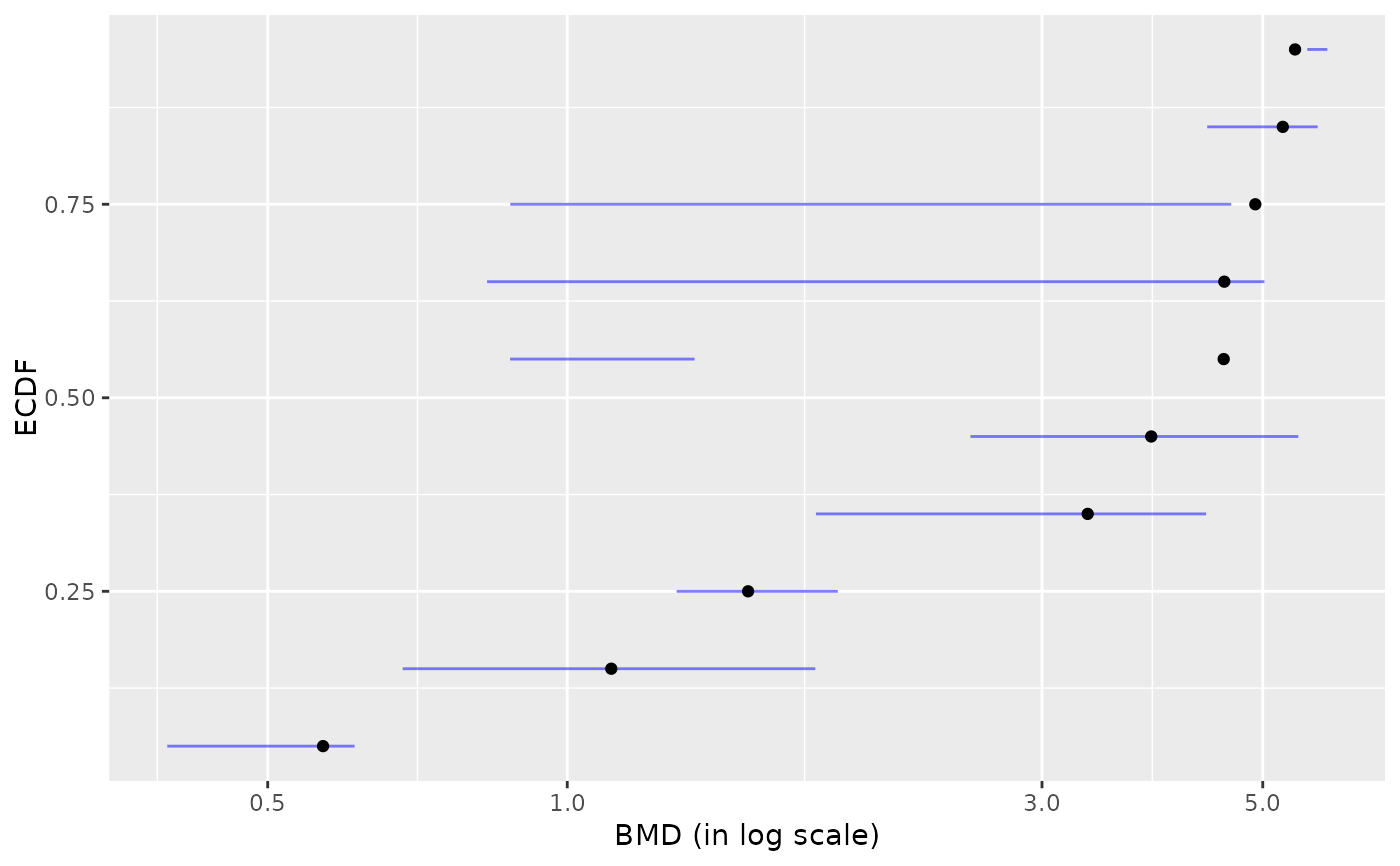
plot(b) # plot of BMD.zSD after removing of BMDs with infinite upper bounds
#> `height` was translated to `width`.
 # \donttest{
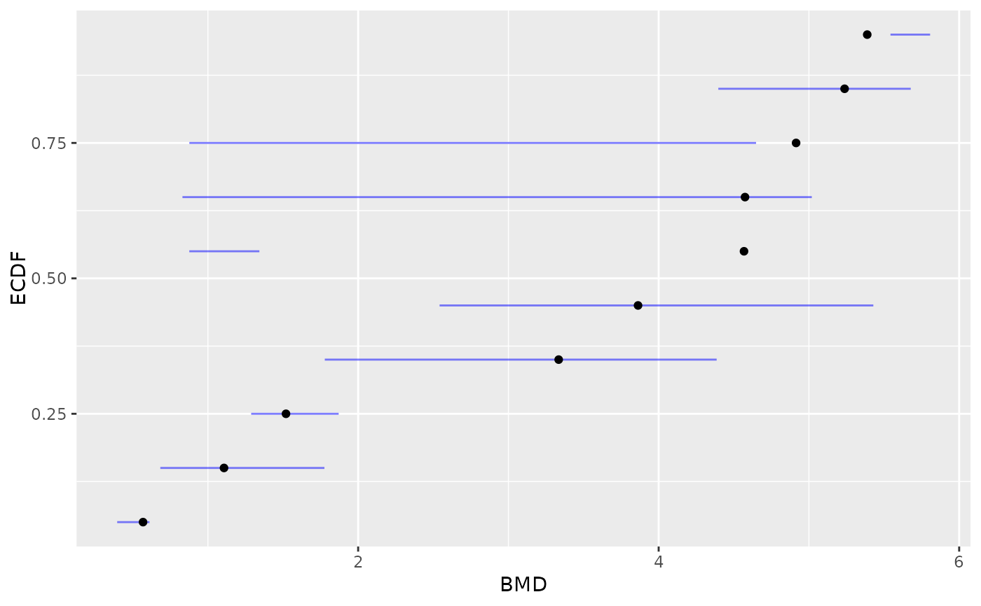
# same plot in raw scale (without log transformation of BMD values)
plot(b, BMD_log_transfo = FALSE)
#> `height` was translated to `width`.
 # plot of BMD.zSD without removing of BMDs
# with infinite upper bounds
plot(b, remove.infinite = FALSE)
#> `height` was translated to `width`.
 # }
# bootstrap on only a subsample of items
# with a greater number of iterations
# \donttest{
chosenitems <- r$res$id[1:5]
(b.95 <- bmdboot(r, items = chosenitems,
niter = 1000, progressbar = TRUE))
#> The bootstrap may be long if the number of items and the number of
#> bootstrap iterations is high.
#>
|
| | 0%
|
|============== | 20%
|
|============================ | 40%
|
|========================================== | 60%
|
|======================================================== | 80%
|
|======================================================================| 100%
#> Bootstrap confidence interval computation was successful on 5 items among5.
#> For 0 BMD.zSD values and 3 BMD.xfold values among 5 at least one bound
#> of the 95 percent confidence interval could not be computed due to some
#> bootstrapped BMD values not reachable due to model asymptotes or
#> reached outside the range of tested doses (bounds coded Inf)).
b.95$res
#> id irow adjpvalue model nbpar b c d
#> 1 15 15 1.546048e-05 exponential 3 0.07142237 NA 7.740153
#> 2 12.1 12 2.869315e-05 Gauss-probit 5 0.41415104 8.903415 7.564374
#> 3 27.1 27 3.087292e-05 linear 2 -0.10844680 NA 15.608419
#> 4 25.1 25 1.597308e-04 exponential 3 -0.12880712 NA 15.142111
#> 5 4 4 2.302448e-04 Gauss-probit 4 3.07918819 9.851210 9.851210
#> e f SDres typology trend y0 yatdosemax
#> 1 2.276377 NA 0.3183292 E.inc.convex inc 7.740153 8.983706
#> 2 1.131878 0.7204104 0.3802228 GP.bell bell 7.585780 8.903415
#> 3 NA NA 0.1648041 L.dec dec 15.608419 14.889308
#> 4 3.404150 NA 0.2142472 E.dec.concave dec 15.142111 14.367457
#> 5 1.959459 -1.6121603 0.2994936 GP.U U 8.534547 9.341173
#> yrange maxychange xextrem yextrem BMD.zSD BMR.zSD BMD.xfold
#> 1 1.2435537 1.2435537 NA NA 3.8627796 8.058482 5.6254804
#> 2 1.5579862 1.5579862 1.438980 9.143766 0.5682965 7.966002 0.7867277
#> 3 0.7191107 0.7191107 NA NA 1.5196769 15.443615 NA
#> 4 0.7746535 0.7746535 NA NA 3.3346126 14.927864 NA
#> 5 1.1021236 0.8066266 1.959459 8.239050 4.9146813 8.834040 NA
#> BMR.xfold BMD.zSD.lower BMD.zSD.upper BMD.xfold.lower BMD.xfold.upper
#> 1 8.514168 1.9234542 5.3597201 4.2884456 6.313835
#> 2 8.344358 0.2471539 0.8194022 0.5083066 1.067867
#> 3 14.047577 0.9228184 2.1008927 Inf Inf
#> 4 13.627900 1.5729443 5.0433579 Inf Inf
#> 5 9.388001 0.5446487 5.1515178 5.7927268 Inf
#> nboot.successful
#> 1 932
#> 2 563
#> 3 1000
#> 4 931
#> 5 745
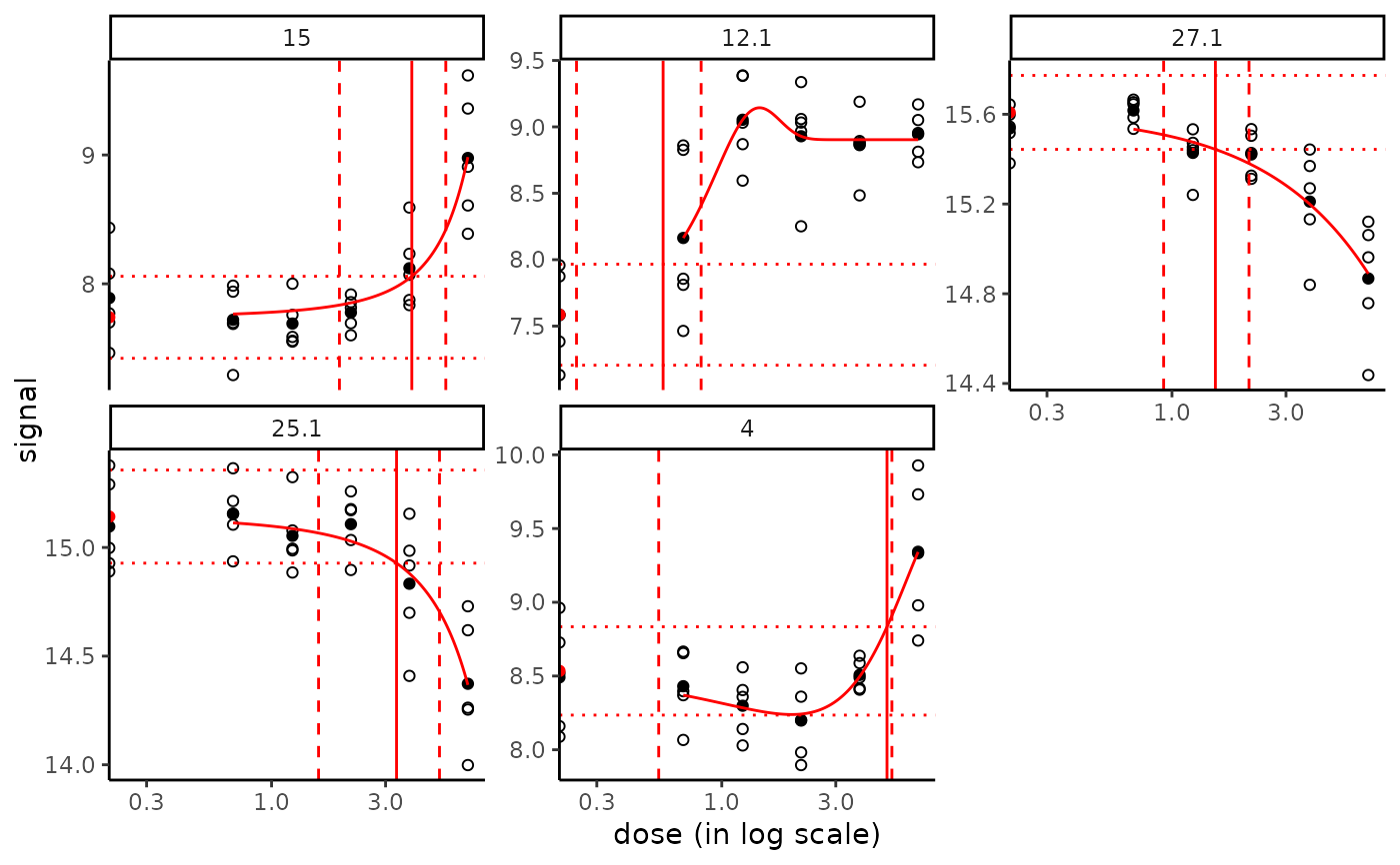
# Plot of fits with BMD values and confidence intervals
# with the default BMD.zSD
plot(f, items = chosenitems, BMDoutput = b.95, BMDtype = "zSD")
#> Warning: log-10 transformation introduced infinite values.
#> Warning: log-10 transformation introduced infinite values.
#> Warning: log-10 transformation introduced infinite values.
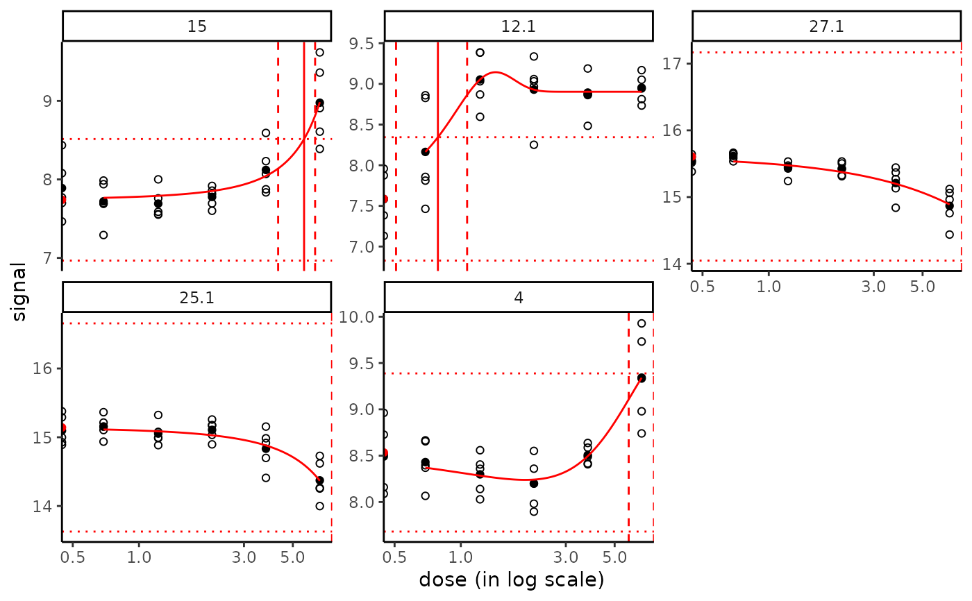
 # with the default BMD.xfold
plot(f, items = chosenitems, BMDoutput = b.95, BMDtype = "xfold")
#> Warning: log-10 transformation introduced infinite values.
#> Warning: log-10 transformation introduced infinite values.
#> Warning: log-10 transformation introduced infinite values.
#> Warning: Removed 3 rows containing missing values or values outside the scale range
#> (`geom_vline()`).
 # same bootstrap but changing the default confidence level (0.95) to 0.90
(b.90 <- bmdboot(r, items = chosenitems,
niter = 1000, conf.level = 0.9, progressbar = TRUE))
#> The bootstrap may be long if the number of items and the number of
#> bootstrap iterations is high.
#>
|
| | 0%
|
|============== | 20%
|
|============================ | 40%
|
|========================================== | 60%
|
|======================================================== | 80%
|
|======================================================================| 100%
#> Bootstrap confidence interval computation was successful on 5 items among5.
#> For 0 BMD.zSD values and 3 BMD.xfold values among 5 at least one bound
#> of the 95 percent confidence interval could not be computed due to some
#> bootstrapped BMD values not reachable due to model asymptotes or
#> reached outside the range of tested doses (bounds coded Inf)).
b.90$res
#> id irow adjpvalue model nbpar b c d
#> 1 15 15 1.546048e-05 exponential 3 0.07142237 NA 7.740153
#> 2 12.1 12 2.869315e-05 Gauss-probit 5 0.41415104 8.903415 7.564374
#> 3 27.1 27 3.087292e-05 linear 2 -0.10844680 NA 15.608419
#> 4 25.1 25 1.597308e-04 exponential 3 -0.12880712 NA 15.142111
#> 5 4 4 2.302448e-04 Gauss-probit 4 3.07918819 9.851210 9.851210
#> e f SDres typology trend y0 yatdosemax
#> 1 2.276377 NA 0.3183292 E.inc.convex inc 7.740153 8.983706
#> 2 1.131878 0.7204104 0.3802228 GP.bell bell 7.585780 8.903415
#> 3 NA NA 0.1648041 L.dec dec 15.608419 14.889308
#> 4 3.404150 NA 0.2142472 E.dec.concave dec 15.142111 14.367457
#> 5 1.959459 -1.6121603 0.2994936 GP.U U 8.534547 9.341173
#> yrange maxychange xextrem yextrem BMD.zSD BMR.zSD BMD.xfold
#> 1 1.2435537 1.2435537 NA NA 3.8627796 8.058482 5.6254804
#> 2 1.5579862 1.5579862 1.438980 9.143766 0.5682965 7.966002 0.7867277
#> 3 0.7191107 0.7191107 NA NA 1.5196769 15.443615 NA
#> 4 0.7746535 0.7746535 NA NA 3.3346126 14.927864 NA
#> 5 1.1021236 0.8066266 1.959459 8.239050 4.9146813 8.834040 NA
#> BMR.xfold BMD.zSD.lower BMD.zSD.upper BMD.xfold.lower BMD.xfold.upper
#> 1 8.514168 2.1636242 5.1282797 4.4988439 6.218120
#> 2 8.344358 0.2862255 0.7638092 0.5877853 1.025521
#> 3 14.047577 0.9791835 2.0226321 Inf Inf
#> 4 13.627900 1.8299433 4.8873535 Inf Inf
#> 5 9.388001 0.6371109 4.9854763 5.9397256 Inf
#> nboot.successful
#> 1 942
#> 2 581
#> 3 1000
#> 4 949
#> 5 769
# }
# (2) an example on a microarray data set (a subsample of a greater data set)
#
# \donttest{
datafilename <- system.file("extdata", "transcripto_sample.txt", package="DRomics")
(o <- microarraydata(datafilename, check = TRUE, norm.method = "cyclicloess"))
#> Just wait, the normalization using cyclicloess may take a few minutes.
#> Elements of the experimental design in order to check the coding of the data:
#> Tested doses and number of replicates for each dose:
#>
#> 0 0.69 1.223 2.148 3.774 6.631
#> 5 5 5 5 5 5
#> Number of items: 1000
#> Identifiers of the first 20 items:
#> [1] "1" "2" "3" "4" "5.1" "5.2" "6.1" "6.2" "7.1" "7.2"
#> [11] "8.1" "8.2" "9.1" "9.2" "10.1" "10.2" "11.1" "11.2" "12.1" "12.2"
#> Data were normalized between arrays using the following method: cyclicloess
(s_quad <- itemselect(o, select.method = "quadratic", FDR = 0.001))
#> Removing intercept from test coefficients
#> Number of selected items using a quadratic trend test with an FDR of 0.001: 78
#> Identifiers of the first 20 most responsive items:
#> [1] "384.2" "383.1" "383.2" "384.1" "301.1" "363.1" "300.2" "364.2" "364.1"
#> [10] "363.2" "301.2" "300.1" "351.1" "350.2" "239.1" "240.1" "240.2" "370"
#> [19] "15" "350.1"
(f <- drcfit(s_quad, progressbar = TRUE))
#> The fitting may be long if the number of selected items is high.
#>
|
| | 0%
|
|= | 1%
|
|== | 3%
|
|=== | 4%
|
|==== | 5%
|
|==== | 6%
|
|===== | 8%
|
|====== | 9%
|
|======= | 10%
|
|======== | 12%
|
|========= | 13%
|
|========== | 14%
|
|=========== | 15%
|
|============ | 17%
|
|============= | 18%
|
|============= | 19%
|
|============== | 21%
|
|=============== | 22%
|
|================ | 23%
|
|================= | 24%
|
|================== | 26%
|
|=================== | 27%
|
|==================== | 28%
|
|===================== | 29%
|
|====================== | 31%
|
|====================== | 32%
|
|======================= | 33%
|
|======================== | 35%
|
|========================= | 36%
|
|========================== | 37%
|
|=========================== | 38%
|
|============================ | 40%
|
|============================= | 41%
|
|============================== | 42%
|
|=============================== | 44%
|
|=============================== | 45%
|
|================================ | 46%
|
|================================= | 47%
|
|================================== | 49%
|
|=================================== | 50%
|
|==================================== | 51%
|
|===================================== | 53%
|
|====================================== | 54%
|
|======================================= | 55%
|
|======================================= | 56%
|
|======================================== | 58%
|
|========================================= | 59%
|
|========================================== | 60%
|
|=========================================== | 62%
|
|============================================ | 63%
|
|============================================= | 64%
|
|============================================== | 65%
|
|=============================================== | 67%
|
|================================================ | 68%
|
|================================================ | 69%
|
|================================================= | 71%
|
|================================================== | 72%
|
|=================================================== | 73%
|
|==================================================== | 74%
|
|===================================================== | 76%
|
|====================================================== | 77%
|
|======================================================= | 78%
|
|======================================================== | 79%
|
|========================================================= | 81%
|
|========================================================= | 82%
|
|========================================================== | 83%
|
|=========================================================== | 85%
|
|============================================================ | 86%
|
|============================================================= | 87%
|
|============================================================== | 88%
|
|=============================================================== | 90%
|
|================================================================ | 91%
|
|================================================================= | 92%
|
|================================================================== | 94%
|
|================================================================== | 95%
|
|=================================================================== | 96%
|
|==================================================================== | 97%
|
|===================================================================== | 99%
|
|======================================================================| 100%
#> Results of the fitting using the AICc to select the best fit model
#> 11 dose-response curves out of 78 previously selected were removed
#> because no model could be fitted reliably.
#> Distribution of the chosen models among the 67 fitted dose-response curves:
#>
#> Hill linear exponential Gauss-probit
#> 0 11 30 23
#> log-Gauss-probit
#> 3
#> Distribution of the trends (curve shapes) among the 67 fitted dose-response curves:
#>
#> U bell dec inc
#> 6 20 22 19
(r <- bmdcalc(f))
#> 1 BMD-xfold values and 0 BMD-zSD values are not defined (coded NaN as
#> the BMR stands outside the range of response values defined by the model).
#> 28 BMD-xfold values and 0 BMD-zSD values could not be calculated (coded
#> NA as the BMR stands within the range of response values defined by the
#> model but outside the range of tested doses).
(b <- bmdboot(r, niter = 100)) # niter to put at 1000 for a better precision
#> Warning:
#> A small number of iterations (less than 1000) may not be sufficient to
#> ensure a good quality of bootstrap confidence intervals.
#> The bootstrap may be long if the number of items and the number of
#> bootstrap iterations is high.
#>
|
| | 0%
|
|= | 1%
|
|== | 3%
|
|=== | 4%
|
|==== | 6%
|
|===== | 7%
|
|====== | 9%
|
|======= | 10%
|
|======== | 12%
|
|========= | 13%
|
|========== | 15%
|
|=========== | 16%
|
|============= | 18%
|
|============== | 19%
|
|=============== | 21%
|
|================ | 22%
|
|================= | 24%
|
|================== | 25%
|
|=================== | 27%
|
|==================== | 28%
|
|===================== | 30%
|
|====================== | 31%
|
|======================= | 33%
|
|======================== | 34%
|
|========================= | 36%
|
|========================== | 37%
|
|=========================== | 39%
|
|============================ | 40%
|
|============================= | 42%
|
|============================== | 43%
|
|=============================== | 45%
|
|================================ | 46%
|
|================================= | 48%
|
|================================== | 49%
|
|==================================== | 51%
|
|===================================== | 52%
|
|====================================== | 54%
|
|======================================= | 55%
|
|======================================== | 57%
|
|========================================= | 58%
|
|=========================================== | 61%
|
|============================================ | 63%
|
|============================================= | 64%
|
|============================================== | 66%
|
|=============================================== | 67%
|
|================================================ | 69%
|
|================================================= | 70%
|
|================================================== | 72%
|
|=================================================== | 73%
|
|==================================================== | 75%
|
|===================================================== | 76%
|
|====================================================== | 78%
|
|======================================================== | 81%
|
|========================================================= | 82%
|
|============================================================ | 85%
|
|============================================================= | 87%
|
|============================================================== | 88%
|
|=============================================================== | 90%
|
|================================================================ | 91%
|
|================================================================= | 93%
|
|================================================================== | 94%
|
|==================================================================== | 97%
|
|===================================================================== | 99%
|
|======================================================================| 100%
#> Bootstrap confidence interval computation failed on 4 items among 67
#> due to lack of convergence of the model fit for a fraction of the
#> bootstrapped samples greater than 0.5.
#> For 0 BMD.zSD values and 36 BMD.xfold values among 67 at least one
#> bound of the 95 percent confidence interval could not be computed due
#> to some bootstrapped BMD values not reachable due to model asymptotes
#> or reached outside the range of tested doses (bounds coded Inf)).
# different plots of BMD-zSD
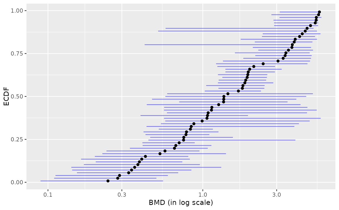
plot(b)
#> Warning:
#> 4 BMD values for which lower and upper bounds were coded NA or with
#> lower or upper infinite bounds were removed before plotting.
#> `height` was translated to `width`.
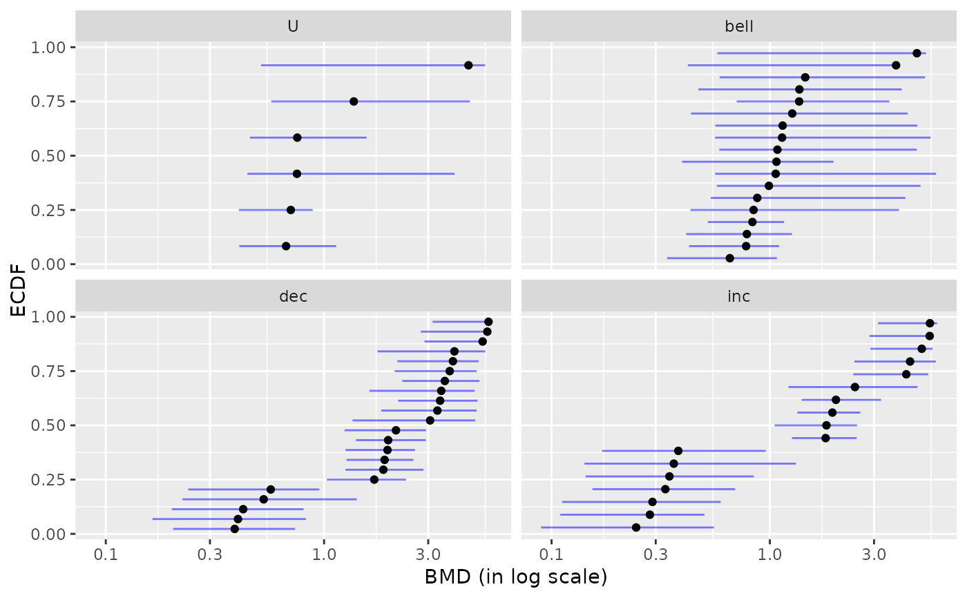
 plot(b, by = "trend")
#> Warning:
#> 4 BMD values for which lower and upper bounds were coded NA or with
#> lower or upper infinite bounds were removed before plotting.
#> `height` was translated to `width`.
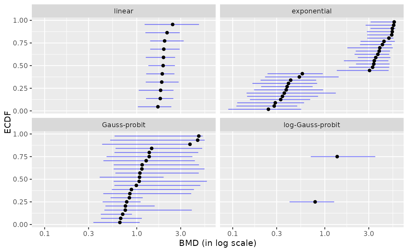
 plot(b, by = "model")
#> Warning:
#> 4 BMD values for which lower and upper bounds were coded NA or with
#> lower or upper infinite bounds were removed before plotting.
#> `height` was translated to `width`.
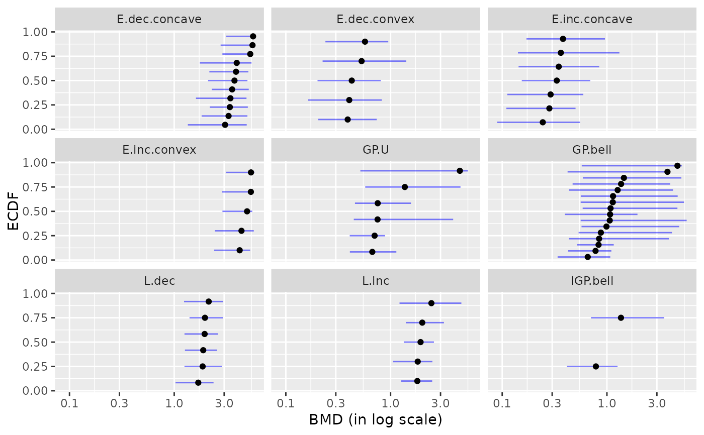
 plot(b, by = "typology")
#> Warning:
#> 4 BMD values for which lower and upper bounds were coded NA or with
#> lower or upper infinite bounds were removed before plotting.
#> `height` was translated to `width`.
 # a plot of BMD-xfold (by default BMD-zSD is plotted)
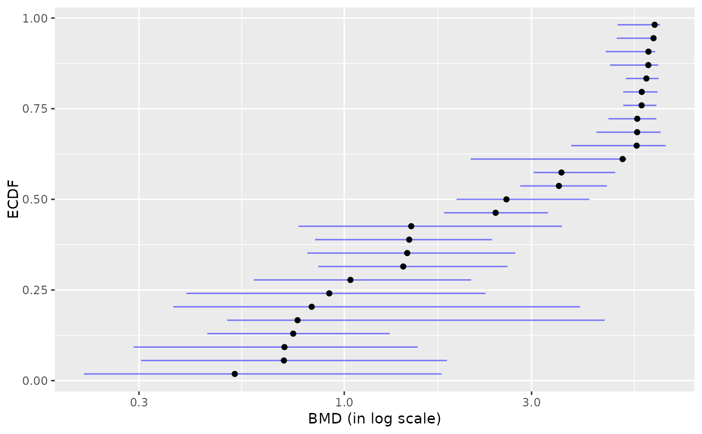
plot(b, BMDtype = "xfold")
#> Warning:
#> 40 BMD values for which lower and upper bounds were coded NA or with
#> lower or upper infinite bounds were removed before plotting.
#> `height` was translated to `width`.
 # }
# (3) Comparison of parallel and non parallel implementations
#
# \donttest{
# to be tested with a greater number of iterations
if(!requireNamespace("parallel", quietly = TRUE)) {
if(parallel::detectCores() > 1) {
system.time(b1 <- bmdboot(r, niter = 100, progressbar = TRUE))
system.time(b2 <- bmdboot(r, niter = 100, progressbar = FALSE, parallel = "snow", ncpus = 2))
}}
# }
# }
# (3) Comparison of parallel and non parallel implementations
#
# \donttest{
# to be tested with a greater number of iterations
if(!requireNamespace("parallel", quietly = TRUE)) {
if(parallel::detectCores() > 1) {
system.time(b1 <- bmdboot(r, niter = 100, progressbar = TRUE))
system.time(b2 <- bmdboot(r, niter = 100, progressbar = FALSE, parallel = "snow", ncpus = 2))
}}
# }